| AutoFEM Analysis Buckling Analysis Steps | |||||||
| AutoFEM Analysis Buckling Analysis Steps | |||||||
Details of Buckling Analysis Steps
Buckling Analysis is performed in several stages. The order of steps for the user to put together a study and run calculations of the structural buckling analysis is mostly similar to the algorithm described for the Static Analysis. Therefore, in this chapter we will just mention what is special for the buckling analysis:
1. Creating Study. When creating a study, specify its type – «Buckling Analysis»
2. Applying boundary conditions. Just like in the static analysis, the buckling analysis uses restraints and loads as boundary conditions. All types of restraints and all types of forces can be used in the buckling analysis. The thermal impact is defined in the same way as in the static analysis. Defining restraints and forces is a necessary condition for running a correct analysis. The combined limitation on the model must satisfy the following condition:
To be suited for a buckling analysis, a model should have restraints preventing free movement in the space as a solid body. Failing to meet this condition will cause incorrect results of Finite Element analysis or abortion of computations. |
Note also that defining loads properly is important for the initial buckling study to be correctly formulated. In particular, in certain loading cases, the solution to the study may not have physical sense (for example, in the case of a rod being stretched with a tensile longitudinal force). Correctly defined boundary conditions are signified by a positive value of the critical load coefficient, resulting from the study.
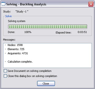
3. Running calculations. Before running calculations, the user specifies computational algorithms and the number of buckling modes to be analysed, in the study properties. The following data is output into the information window when running calculations:
Nodes - the number of nodes in the computational finite element mesh.
Elements - the number of tetrahedrons in the finite element mesh.
Arguments – the number of equations used in the calculation.
Calculation complete – this message signifies that the solution process is completed successfully.
4. Results. The following are analysis results:
Load Factor – the calculated value of the coefficient, the product of which and the loads applied to the system makes the factual value of the critical load, which brings the system into a new equilibrium state. For example, a distributed force of 1000 Н is applied over the model. The Load Factor, as calculated, is equal to 109.18 . That means, that the first mode of an equilibrium state for the given model has the critical load equal to 109,180 Н.
Load Factor must be positive. If calculations have resulted in a negative Load Factor, that means, no buckling can be produced by the loads applied to the structure.
Relative displacements, corresponding to a given critical load. This type of result reflects on a buckling mode of the structure corresponding to a certain critical load. The buckling modes displayed in the postprocessor window after completing calculations are relative displacements. By analysing those modes, you can make a conclusion about the pattern of displacements in a buckling condition. By knowing the expected buckling mode under a certain critical load, one could, for example, introduce an additional restraint or a support in the part of the structure corresponding to the maximum of buckling in this mode, which would effectively alter mechanical properties of the product.
As an additional (reference) result, you can also output displacements of the structure under the applied static loads, whose calculations preceded the evaluation of the critical load factors.
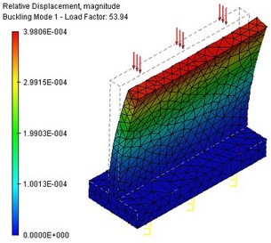
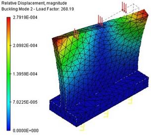
Buckling modes, corresponding to the first and second critical loads on the part
Algorithm for Buckling Analysis Based on modelling
Once the study calculation completes successfully, you should analyse solution results in order to make conclusions on probabilistic buckling of the structure based on results of Finite Element modelling. A typical sequence of steps for validating the results of Finite Element modelling of initial buckling is as follows:
1. Solution evaluation. As was mentioned earlier, the Load Factor must be positive. If the factor came out negative, that means the loads applied to the structure do not produce system buckling.
2. Load factor evaluation. If the Load Factor is positive and is less than 1, that means system buckling will occur under the specified loads, and that the design of the structure needs enhancement. If the Load Factor is positive and is greater than 1, that means there is no buckling threat for the structure under the specified loading conditions.
3. Buckling modes analysis. In the studies tree, use the context menu command "Open" or "Open in new window" to open the "Buckling mode 01" solution, corresponding to the smallest critical loading. We can visually estimate the pattern of the strained state of the structure. The buckling analysis allows making a conclusion about directions and locations of maximum displacements, corresponding to a critical load. This information can be used for optimizing the product's design with the purpose of increasing its resistance to buckling.