Examples of Thermal Analysis Studies

Thermal Analysis of a Cooling Radiator. Steady State

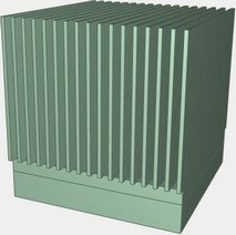
Required is an evaluation of a passive cooling radiator efficiency for the semiconductor electronic device with the maximum dissipating power of 15 Watt. The permissible temperature of the microchip's body is 75°C in the operating range of ambient temperatures from 25°C to 55°C.  An aluminum alloy radiator is used for cooling the device and is mounted at the top of the microchip's body. To improve heat dissipation, the body of the microchip is also made of aluminum.

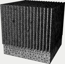
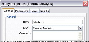
Step 1. Creating «Study», meshing, and assigning material. Create a study of the «Termal Analysis» type using the command «Analysis|New Study» based on two bodies – the microchip and the radiator. Generate a finite element mesh. You also need to define parameters of the part's material. By default, calculations use material properties «From Operation», that is, the material properties are automatically obtained from the product part's solid model. This is especially convenient when a study includes bodies from different materials representing parts of assembly models. In our case, the «Aluminum» material was defined at creation of the 3D model of the radiator and the microchip, with its physical and chemical properties contained in the AutoCAD database.

 

Step 2. Applying boundary conditions. Let us specify thermal loads for the model. We will apply the «Heat power» load of 15 Watt to the volume of the microchip, and define the «Convection» boundary condition on the external heat-sinking radiator surfaces with the convection parameter of 15 Watt/(m2 . °C) and ambient temperature of (25°C). We can disregard in this study the heat exchange factor of mutual and ambient radiation, since their radiation contribution is vanishingly small at the expected temperatures (tens of degrees Celsius). Upon completing the commands of building the finite element mesh and defining thermal loads, we get a calculations-ready finite element model.

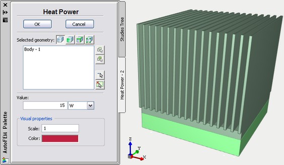
Defining "Heat Power" load

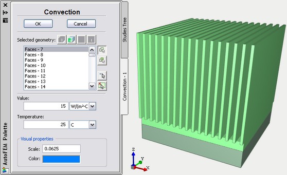
Defining "Convection" load

 

Step 3. Running calculations and analysing results. We will start the thermal analysis by running the command «Analysis|Solve». In the appearing dialogue of the study's properties, set the «Steady state» option on the [Parameters] tab. Use the «Calculate using linear element» mode on the [Solve] tab to speed up the calculations.

The list of calculation results is displayed in the «Studies» window, and can be accessed by the context menu in the calculation results window. The maximum temperature according to the heat and analysis results is 39,1°C at the convection temperature equal to 25°C. We will then edit the convection temperature using the «Edit» command of the studies tree context menu, setting the operational ambient temperature to its upper limit (55°C), and then rerun calculations. We will obtain the maximum temperature of the microchip equal to 69.1°C. The conclusion is the radiator does fulfill the required temperature condition for the device in the entire specified range of the device's operational temperatures. The study is complete.

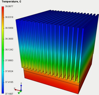
Temperature fields in the radiator under the convection temperature of 25°C

 

Calculating the Time of Heating up the Cooling Radiator. Transient Mode

Let us estimate the time required for the device to reach a steady thermal state. To do this, let's run a transient thermal analysis of the «microchip+radiator» system.

Step 1. Creating study's copy. We will create a copy of the original study in a steady-state thermal analysis using the «Copy» command of the studies tree context menu. On the [General] tab of the study's properties, change the study name to «Heating».

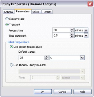
Step 2. Defining parameters of transient analysis. On the [Parameters] tab of the thermal analysis properties, set the «Transient» mode. Define the time analysis parameters – the modelling time of 30 minutes and the modelling step of 0.5 minutes. We will use the uniform ambient temperature (25°C) as the initial model temperature.

Defining calculation parameters of transient heat analysis – time and initial temperature

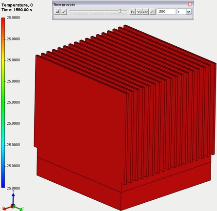
Step 3. Running calculations and analysing results. After the completion of calculations, you can examine results at each time step. To view such results, we use a floating «Time process» bar that allows the user to quickly switch to the time instant of interest using a slider. With the help of these tools we determine that a nearly complete heating of the radiator will occur after approximately 26 minutes.

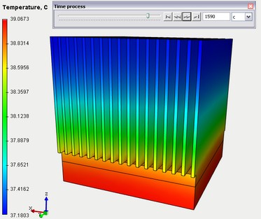
Result of thermal analysis at time 1590 sec (26 min.)

 

Calculating Time of Cooling down the Cooling Radiator. Transient Mode

Now, let's evaluate the time required for the device-cooling radiator to cool down after an extended work.

Step 1. Creating study's copy. Adjusting boundary conditions. Let's create a copy of the original study of the steady-state thermal analysis. Adjust the boundary conditions of this study: the «Heat power» load will be deleted.

Step 2. Defining parameters of transient analysis. Set the «Transient» mode on the tab of the thermal analysis properties. Define time analysis parameters – the modelling time of 30 minutes, the modelling step of 0.5 minutes. Let's use the result from the previous steady-state radiator evaluation as the initial model temperature.

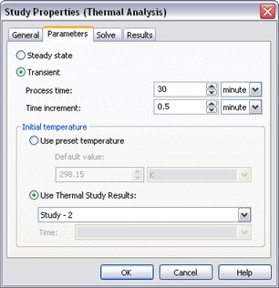
Setting up study parameters for calculating cooling process

(transient heat transfer)

Step 3. Analysing calculation results. Let's run calculations and analyse the results. Using the «Time process» bar, we can determine that nearly complete cooling of the radiator will occur in approximately 26 minutes after turning the device off.

Device cooling calculation.

Temperatures distribution at 1590 seconds of the calculation time

 

 

Return to contents

autofem.com