Details of Static Analysis Steps

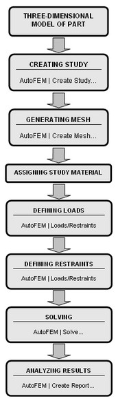
Static Analysis of a model is performed in several stages. Listed are the elements required for conducting an analysis.

To run a static analysis, complete the following steps:

Step 1. Creating three-dimensional solid model of a part.

Before you start working in AutoFEM system, you should prepare a three-dimensional solid model to be evaluated. A solid model can be built in AutoCAD environment or imported from other systems. Static analysis can be performed over one or multiple operations-bodies.

Step 2. Creating "Study".

You can use one of the following ways to create study:

You also need to specify the type ("Static Analysis") of the study in the command's properties window.

If there are multiple bodies in the scene, then you need to select one or several contacting bodies, for which a new study will be created.

Step 3. Defining material.

One of the required elements of any solution is the study's material. Detailed description of material defining methods for calculations is provided in the respective section of the preprocessor description.      

Step 4. Creating mesh.

To perform Finite Element modelling, you need to construct a finite element mesh. By default, the mesh construction command initiates automatically when creating a study. The user can also create a mesh using the AutoFEM command " AutoFEM | Create Mesh...". When creating a mesh, the user defines various parameters of discretizing a solid-state model. The finite element mesh can significantly influence the quality of the obtained solution in the cases of complex spatial configuration of parts. The finite element mesh generation parameters are reviewed in detail in the respective section of AutoFEM preprocessor description.

Step 5. Applying boundary conditions.

In static analysis, boundary conditions are represented by restraining methods and external loads applied to the system. The boundary conditions creating stage is very important and requires good understanding by the engineer of the essence of the study being solved. Therefore, think over the physical aspects of the study thoroughly before applying boundary conditions.

Defining restraints is a necessary condition for running a correct static analysis. The combined limitation on the body movement must satisfy the following condition:

To be suited for a static analysis, a model should have restraints preventing free movement in the space as a solid body. Failing to meet this condition will cause incorrect results of Finite Element analysis or abortion of computations.

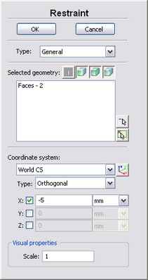
A command is provided in AutoFEM for defining restraints: "Fixture". The "Fixed" type of the restraints defines a fully fixed (immovable) state for the selected model element. The "General" type of the restraints allows to limit model element motion along the axes of the chosen coordinate system.

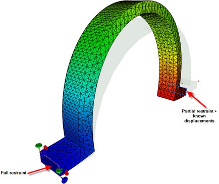
The "Fixture" command also provides another useful functionality. There is a resource to specify known displacements for the structure in it. For this, specify the value of fixed displacement of a model element along some of the coordinate axes in the "Fixture" command's properties window. Static Analysis will be performed with this condition accounted for. Note that a static solution is possible in this case without applying additional (force) loads. In this way, one can evaluate the stress developing in a strained structure when the quantitative values of the strain (displacements) are known.

A number of specialized commands is provided in AutoFEM to define loads; those allow to define main types of loads ("Force", "Pressure", "Centrifugal Force", "Acceleration", "Bearing Load", "Torque"). Detailed description of all types of loads is provided in the preprocessor description.

Note one more functional capability of a static solution in AutoFEM. The user can define a structure's stress state analysis not only under various forces, but also under thermal loads - the "Thermoelasticity" Study. As known, structural materials develop linear strain under the thermal impact - expand under heating and shrink under cooling. Changes in a body's dimensions cause strain and a stressed state. AutoFEM accounts for changing temperatures. To define temperatures when accounting for transient temperature fields, use the command:

At the same time, you need to enable the "Consider Thermoeffects" option on the [Thermoelasticity] tab of the static study parameters dialogue in order to account for thermal loads in the static solution. You will also need to define the temperature of "zero" strain, which corresponds to the no-stress state of the model, and to define the working temperature field (details are in the section "Settings of Linear Statics Processor").

Step 6. Running calculations.

Once a finite element mesh is built for the model and boundary conditions are applied (restraints and loads), you can start the process or creating and solving linear algebraic equations of the static analysis. Use the following command to start solving the active study:

The selected study's calculation can be started from the context menu by clicking on the name of the selected study in the studies tree.

By default, the "Study parameters" dialogue of the static analysis opens automatically before calculations. In this dialogue, the user can define the desired options and settings of the solution, as well as specify the types of solution data displayable in the studies tree. Detailed description of study settings purpose is further available in the section "Settings of Linear Statics Processor". Most of the settings are selected by the processor automatically depending on the number of dimensions in the study being solved and imposed boundary conditions.

Clicking the [OK] button in the study parameters dialogue launches the process of building and solving systems of linear algebraic equations. The stages of solving equations and additional reference information are displayed in a special information pane. Clicking the [Close] button in the information pane terminates calculations. The "Close this dialogue box on solving complection" flag will force automatic closing of the solution steps monitoring window after finishing solving equations.

The flag «Save Document on solving completion» will force automatic saving of calculation results and all changed data in the active document.

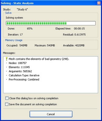
The following reference data is output in the information window:

Nodes - the number of nodes in the computational finite element mesh.

Elements - the number of tetrahedrals in the finite element mesh.

Arguments - the number of equations of linear statics.

Calculation Type - the algorithm used for solving equations. Types of possible algorithms and their use are described in the section "Settings of Linear Statics Processor".

Solution Found – tells that system of equations was successfully calculated. There is also auxiliary information in the brackets: iter – number of executed iteration (if iterative method was used), tol – miscalculation of result after calculation.

For the iteration solver, the number of the current iteration and the residual error of the solution are presented. For the direct method, the percentage of the total number of the solved equations is shown. The user can see in the real-time mode, what is the rate of solving equations, and manage this process. In addition, for both solving methods, three parameters are shown, which characterize the need in operational memory: what amount of memory is occupied by the solver at present; maximum usage; and how much free operational memory is available in the system just now. These parameters allow each user to assess whether his/her computer system fits the solution of a particular problem.

The calculation steps are also visually displayed as a dynamically updating scale. Additionally, the time elapsed from the start of calculations is shown. After finishing calculations, the user must close the auxiliary window (unless the auto close option is enabled).

Step 7. Analysis of static solution results.

After completing calculations, a new "Results" folder appears in the studies tree. By default, this one displays the results defined on the "Results" tab of the "Study parameters" dialogue. Overall, the user can access 38 solutions in the result of the static analysis, sorted out into 6 groups.

"Displacements" group includes the following results.

- Component of displacement vector for a node of the finite element mesh along the OX-axis of the global coordinate system;

- Component of displacement vector for a node of the finite element mesh along the OY-axis of the global coordinate system;

- Component of displacement vector for a node of the finite element mesh along the OY-axis of the global coordinate system.

Displacements, absolute value – the absolute value of the nodal displacements of the model, defined for each node according to the formula:, where x, y, z - displacement vector components for the i-th node of the finite element mesh.

Group «Stresses» includes the following results:

- relative equivalent stresses evaluated from components of the stress tensor according to the formula:;

- normal stress in the direction of the OX-axis of the global coordinate system;

- normal stress in the direction of the OY-axis of the global coordinate system;

- normal stress in the direction of the OZ-axis of the global coordinate system;

- shear stress acting in the direction of the OY-axis of the global coordinate system on a plane with the normal vector parallel to the OX-axis;

- shear stress acting in the direction of the OZ-axis of the global coordinate system on a plane with the normal vector parallel to the OX-axis;

- shear stress acting in the direction of the OZ-axis of the global coordinate system on a plane with the normal vector parallel to the OY-axis;

- principal stresses .

Stress intensity is defined in the following way:

 

Stress error estimation. This result displays the estimation of stress calculation error in percents. The estimation is plotted as element value (constant within a single tetrahedron). Big error value of the element signifies  that there is the big difference in stress calculation with its neighboring elements. The most reliable result of stress calculation is achieved when stress error estimation tends to uniform distribution. For more information about error estimation, refer to International Journal for Numerical Methods in Engineering, vol. 24, 337-357 (1987) “A Simple Error Estimator and Adaptive Procedure for Practical Engineering Analysis” by O.C. Zienkiewicz and J. Z. Zhu)..        

 

Group «Safety factor by stresses» includes the following results:

Safety factor by equivalent stresses represents the ratio of admissible for a given structural material stresses [σ ] to the equivalent stresses:

Safety factor by shear stresses is evaluated as:

Safety factor by normal stresses is evaluated as:

A material's safe stress is defined in the material properties in the standard AutoCAD library or in the appropriate field of the study's materials library. The yield limit is accepted as the safe stress for plastic materials.

Group «Deformation» includes the following results:

- relative equivalent strains expressed in terms of components of the strain tensor by the formula:

;

- relative normal strain in the direction of the OX-axis of the global coordinate system;

- relative normal strain in the direction of the OY-axis of the global coordinate system;

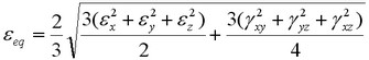- relative normal strain in the direction of the OZ-axis of the global coordinate system;

- shear strain in the OXY plane;

- shear strain in the OXZ plane;

-shear strain in the OYZ plane.

- principal strains .

Strain Energy Density. The result reflects volume distribution of strain energy over the model.

Group «Reactions». The result reflects forces building up in the supporting (fixed) nodes of the finite element model.

-reaction force in the direction of the OX-axis of the global coordinate system;

- reaction force in the direction of the OY-axis of the global coordinate system;

- reaction force in the direction of the OZ-axis of the global coordinate system;

Reaction force (absolute value) – the magnitude of the absolute value of the nodal reaction forces of the model defined for a node as , where - x-component, - y-component, – z-component of the reaction force for the i-th node of the finite element mesh.

 

 

 

“Total Load” group displays the loads applied to a finite-element model as the effective node responses. This type of data represents reference information.

Temperature. This result shows distribution of temperature field over the volume of the model.

Static analysis algorithm

 

Algorithm for Static Strength Evaluation Based on modelling

Once the study calculation is completed successfully, you should analyse obtained results in order to make conclusions on probabilistic static strength of the structure. In most cases, three types of solution suffice - displacements, stresses and the strain safety factor. A typical sequence of steps for validating the results of Finite Element modelling is as follows:

1.Displacement Analysis. In the studies tree, use the context menu command "Open" or "Open in new window" to open the "Displacement, magnitude" solution. We can visually estimate the pattern and the ranges of the stress-strain state of a structure. It is necessary to analyse displacements in order to verify correctnes of applied loads and to assert correctness of the found solution as a result of solving systems of equations. If the results of displacements analysis indicate that a solution to the study is found and the pattern of the structure's strain state matching the expected, then you can proceed to the next step.

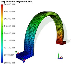
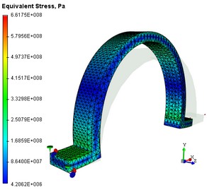
The diagram of absolute displacements and equivalent stresses

2.Stress Analysis. Open the "Equivalent Stress" result. One can visually assess the pattern of the calculated equivalent stress. The stress gradients are illustrated by colour transitions. The colour code scale displayed in the calculation results view window helps reading the approximate value of the displayed result. If you point the mouse to the area of interest on the model, then a tooltip will pop up, displaying the value of the evaluated measure, interpolated by the nearest nodes around the pointer location. The "Equivalent stress" result lets the user make the following conclusions:
a) Determine, at what locations and in which elements of the structure the largest stress develops;
b) By comparing the maxima of the calculated stresses with the allowable stress for the model material, one can assess the degree of the structural strength.

3.Safety factor estimate. Open the "Factor of safety by equivalent stress" result. This result allows estimating the quantitative ratio of the safe stress to the calculated equivalent stresses specified in the material properties. By default, the result is shown on the logarithmic scale in order to reduce the range of colour gradients. If the ratio of the safe and calculated stresses approaches one or becomes less than that, then the strength criterion no longer holds and, therefore, the design must be altered.

 

 

 

Return to contents

autofem.com