
Comparative Benchmarks
To illustrate the AutoFEM Analysis performance, we show several comparative benchmarks comparing the solving time and peak memory consumption of AutoFEM, Ansys and SolidWorks Simulation.
Parameters of the computer system:
Processor - Intel(R) Core(TM)2 Duo CPU E8400 @ 3.00GHz
Random Memory - 8 Gb, DDR2 333 MHz
The best result in the tables is marked with green colour.
Linear Static Analysis
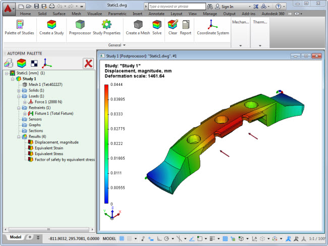
AutoFEM Analysis
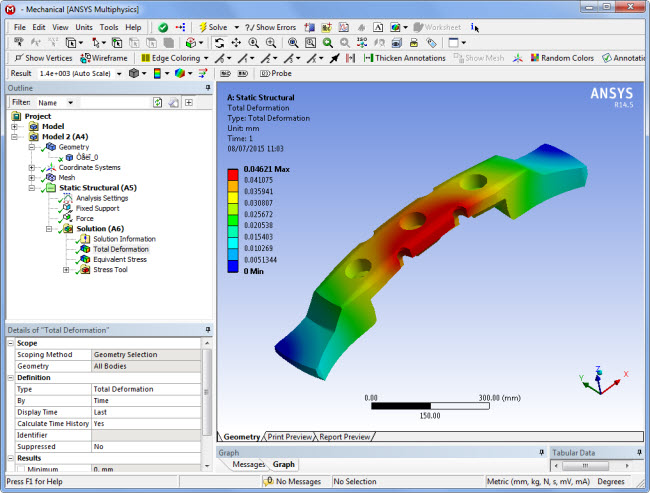
Ansys WorkBench
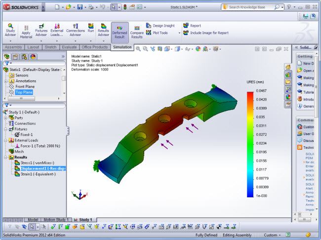
SolidWorks Simulation
Linear Static Analysis, iterative solving method
| CAE System |
Number of elements |
Number of equations |
Solving time, s |
Peak Memory Usage, MB |
| AutoFEM Analysis | 402,227 | 1,689,282 | 81 | 2,070 |
| Ansys WorkBench | 399,329 | 1,648,450 | 169 | 1,600 |
| SolidWorks Simulation | 406,836 | 1,749,819 | 79 | 950 |
Linear Static Analysis, direct solving method
| CAE System |
Number of elements |
Number of equations |
Solving time, s |
Peak Memory Usage, MB |
| AutoFEM Analysis | 44,621 | 209,499 | 17 | 1,211 |
| Ansys WorkBench | 44,627 | 233,421 | 33 | 1,620 |
| SolidWorks Simulation | 44,487 | 204,150 | 46 | 1,220 |
Frequency Analysis
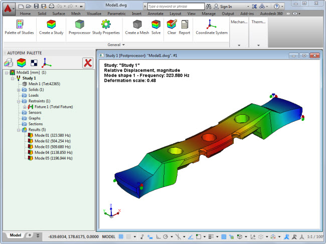
AutoFEM Analysis
Ansys WorkBench
SolidWorks Simulation
Frequency Analysis, iterative solving method, 5 modes
| CAE System |
Number of elements |
Number of equations |
Solving time, s |
Peak Memory Usage, MB |
| AutoFEM Analysis | 42,983 | 199,314 | 39 | 430 |
| Ansys WorkBench | 41,410 | 216,573 | 57 | 1,773 |
| SolidWorks Simulation | 42,679 |
195,750 |
58 | 116 |
Frequency Analysis, direct solving method, 5 modes
| CAE System |
Number of elements |
Number of equations |
Solving time, s |
Peak Memory Usage, MB |
| AutoFEM Analysis | 44,621 | 209,499 | 43 | 1,210 |
| Ansys WorkBench | 44,627 | 233,421 | 39 | 1,772 |
| SolidWorks Simulation | 44,487 | 204,150 | 46 | 1,009 |
Buckling Analysis
AutoFEM Analysis
Ansys WorkBench
SolidWorks Simulation
Buckling Analysis, iterative solving method, 5 modes
| CAE System |
Number of elements |
Number of equations |
Solving time, s |
Peak Memory Usage, MB |
| AutoFEM Analysis | 170,267 | 1,005,393 | 207 | 2,018 |
| Ansys WorkBench | 171,521 | 978,597 | n/a | out of memory |
| SolidWorks Simulation | 172,744 |
948,666 |
250 | 3,192 |
Buckling Analysis, direct solving method, 5 modes
| CAE System |
Number of elements |
Number of equations |
Solving time, s |
Peak Memory Usage, MB |
| AutoFEM Analysis | 33,994 | 204,414 | 26 | 811 |
| Ansys WorkBench | 33,808 | 205,500 | 57 | 1,920 |
| SolidWorks Simulation | 33,565 | 209,838 | 42 | 1,009 |
Conclusion.
AutoFEM Analysis provides the calculation performance of the same level as other famous CAE systems.
AutoFEM and other CAE systems comparison
( AutoFEM vs Ansys & SolidWorks Simulation )
We are often asked, "Does AutoFEM provide an acceptable precision of calculations? Is there any comparison AutoFEM and other famous finite element software systems?"
Below you can find a comparison of our tutorial examples, solved, besides AutoFEM, in two other well known finite element systems: ANSYS Workbench and SolidWorks Simulation (CosmosWorks).
Linear Static Strength Analysis
The result "Displacements" in AutoFEM Analysis:


The result "Displacements" in SolidWorks Simulation:


The result "Displacements" in Ansys Workbench:


Comparison:
|
Ansys |
CosmosWorks | ||
| Max Displacements, mm | 0,06497 | 0.06424 | 0.06406 | |
| Number of tetrahedra | 9,924 | 10,797 | 10,601 |
Conclusion:
We can see, the maximal displacements are very close in spite of the difference between finite element meshes.
The result "Stresses von Mises" in AutoFEM Analysis:

The result "Stresses von Mises" in SolidWorks Simulation:

The result "Stresses von Mises" in Ansys Workbench:


Comparison:
|
Ansys |
CosmosWorks | ||
| Max Stresses, MPa | 67,96 | 81,336 | 99,387 |
|
| Number of tetrahedra | 1,281 | 840 | 1,105 |
Conclusion:
We can see fairly large disturbance in stress estimations between all FEA systems because of the finite element mesh coarseness.
Frequency Analysis (determining resonance frequencies)
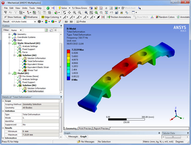
First mode, AutoFEM Analysis:


First mode, Ansys WorkBench:

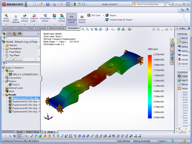
First mode, SolidWorks Simulation:


Fifth mode, AutoFEM Analysis:

Fifth mode, Ansys WorkBench:

Fifth mode, SolidWorks Simulation:


Comparison:
|
Ansys |
CosmosWorks | ||
| First frequency, Hz |
441.92 |
440.13 |
438.84 | |
| Fifth frequency, Hz | 2,853,14 | 2,843.6 | 2,840.3 | |
| Number of tetrahedra | 1,281 | 870 |
1,105 |
Conclusion:
We can see that frequencies and shapes of modes are very close in all systems.
Buckling Analysis (critical load factor)
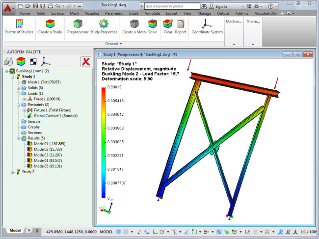
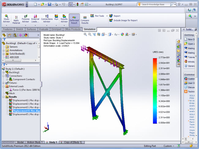
First buckling mode, AutoFEM Analysis:

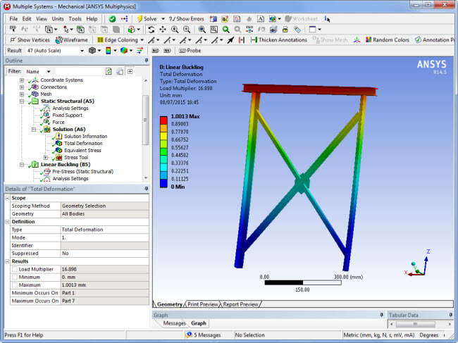
First buckling mode, Ansys WorkBench:

First buckling mode, SolidWorks Simulation:

Third buckling mode, AutoFEM Analysis:

Third buckling mode, Ansys WorkBench:


Third buckling mode, SolidWorks Simulation:


Comparison:
|
Ansys |
CosmosWorks | ||
| First Load Factor |
8.676 |
8.5485 |
8.4937 | |
| Third Load Factor | 16.002 | 15.931 | 15.861 | |
| Number of tetrahedra | 3,209 | 2.871 |
3,103 |
Conclusion:
We can see that all critical-load factors and buckling shapes are very close in all systems.
Thermal Analysis
Temperature field, AutoFEM Analysis:


Temperature field, Ansys WorkBench:


Temperature field, SolidWorks Simulation:


Thermal Flux, AutoFEM Analysis:


Thermal Flux, Ansys WorkBench:


Thermal Flux, SolidWorks Simulation
: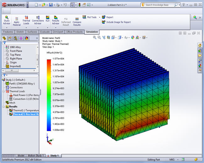
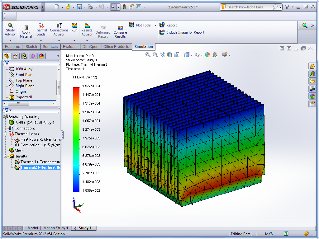
Comparison:
|
Ansys |
CosmosWorks | ||
| Maximum Temperature, C |
38.9824 |
39.088 |
38.996 | |
| Maximum Heat Flux, W/m2 |
14,960 | 19,969 | 15,770 | |
| Number of tetrahedra | 8,710 | 20.776 |
3,103 |
Conclusion: Temperatures and thermal (heat) fluxes are close in all systems.
AutoFEM Analysis Processor
The AutoFEM Analysis Processor is the main engine and brain of the system. Its function is the generation and solving systems of algebraic equations which are derived from the finite element discretization. The AutoFEM Analysis Processor has all necessary possibilities for solving linear and non linear equation systems. It uses as direct methods as well iterative methods. When necessary (in case of big systems or weak computer systems), the mode of using the disk storage turns on.

Window of settings for the static analysis solver.
Stages of solving equations and additional background information are displayed in a special information window, which indicates parameters of the finite element mesh (the number of nodes and elements), the method of solving the system of equations (direct or iterative), the order of iteration for non linear system solving, error messages and etc.

AutoFEM Processor window of the system messages.
Upon completion of calculations, a folder containing its results is created in the tree of the study in AutoFEM Palette window. These results are available for view and analysis by means of the AutoFEM Analysis Postprocessor.
AutoFEM Community
Small and medium companies and educational institutions as well - all select AutoFEM Analysis for finite element modelling.

Most of our users mark the following benefits:
- easiness of use and learning;
- very attractive prices for perpetual licence;
- integration with AutoCAD and ShipConstructor software.


![]()


Testimonials
Borys Sukhanyuk, structural and calculations engineer of Skipskompetance
"I like your program very much. Interface is very nice, logic and very easy to understand and use. All operations are intuitive and easy to perform. Extremly short training time.
I am using AutoFem mostly for check of ShipConstructor structures as well as analysis of solid models where capabilities of beam analysis programs are insufficient.
Analysis can be set up quick and easy."
Volker Junicke, Logistikberatung Dipl.-Ing. (FH)
"Ich bin sehr zufrieden mit der Software. Man muss sich aber Zeit dafür nehmen, um ein gutes Ergebnis zu erzielen und oft viele Experimente durchführen, bis man ein brauchbares Netz erstellt hat."
"I am very satisfied with the software. Though, one must take time to achieve a good result and often perform many experiments until you have created a usable network."
AutoFEM Analysis Postprocessor
At the last stage of the finite element modelling there is a review and analysis of results. Within the framework of AutoFEM Analysis Postprocessor the available results are displayed in the "Palette of Studies" (folder "Results"). The user can change the list of results he/she needs to display by using the "Results" command in the contextual menu.
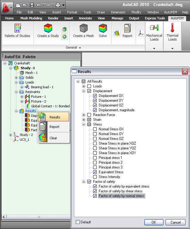
It is possible to open several windows for some of the different results.

Visualization of the results can be flexibly configured using the option dialog in the Postprocessor window. The user can set colors, the scale of the deformed model grid, boundary conditions, loop models, etc. Adjusting the colour scale is needed if you want get a more expressive representation of results.

Options dialog of postprocessor window.
The user has vast possibilities of setting up display numeric values. You can use several predefined types of color scales, and also have the unique opportunity of flexible adjustment of the scale of any color filling. There is opportunity to establish user-defined minimums, maximums and flexible font settings.

Setting window of the color scale.
Often it is needed to analyze the results obtained within the 3D model. To do this, use the command “Section”, which allows you to create a sliced model with the desired angle and view the results.

Cross section on stress diagram.
AutoFEM Analysis Postprocessor has an unique opportunity of a dynamic view of the numerical results by means of moving the mouse over the surface of the deformed finite element model, i.e., sensing. There is also command “Extreme Labels” which shows the points with the maximum and minimum of the resulting value.

Using the extreme and floating labels for indicating the result's value.
The user can create .avi file with the animated result. This movie can be send to the customer to illustrate the result of the finite-element analysis or to be used for better understanding of physical phenomena and for educational purposes, too. It is possible to create a "Report", which is independent of AutoFEM Analysis electronic document and containing basic information about the study. The report is generated in html-format; viewing is possible in any browser, for example, MS Internet Explorer.

Creating a report in html format.
Thus, AutoFEM Analysis has a vast potential of analyzing the results of the finite element analysis and of their representation for customers; also it might be used in the production sector of economy.
You can see it yourself using