Integration of AutoFEM Analysis with ShipConstructor
Based on AutoCAD, ShipConstructor is the leading software product for ship design and ship building, adopted worldwide. ShipConstructor provides the tools needed to design, model and prepare production documentation for any type of vessel, be it a ship, a submarine or an offshore platform.
In the course of designing a vessel or an offshore structure, it is necessary to verify its strength and stiffness characteristics, preferably using Finite Element Analysis. Thanks to direct integration of AutoFEM Analysis and AutoCAD, ShipConstructor users can now use apply AutoFEM to transparently run FEA analysis of ShipConstructor models.
As of AutoFEM Analysis v2.2, the integration with ShipConstructor is complete. The ShipConstructor 2014 stock catalogue supports the mechanical properties of materials needed for FEA, and AutoFEM reads the full model topology directly, including:
Names of parts
• Names of AutoCAD layers (for parts in the current document)
• Data about the material (name, grade, etc.). If the user has not specified thee, they will be taken from the native AutoFEM Analysis materials library, using a name matching technique.

Settings of integration with ShipConstructor

ShipConstructor parts and all related information are acquired by AutoFEM Analysis, and
if needed, ShipConstructor materials are name-matched with materials in the AutoFEM library.
Calculation example of a ShipConstructor Assembly
Download tutorial video about AutoFEM & ShipConstructor integration
Detailed article about joint work of AutoFEM & Shipconstructor (pdf)
AutoFEM Analysis & ShipConstructor Software: Working Together
AutoFEM Analysis & ShipConstructor Software: Working Together
AutoFEM Analysis (AutoFEM Software, United Kingdom)
Joint use of AutoFEM Analysis and ShipConstructor software
ShipConstructor&AutoFEM: How does it work?
Preparation of the calculation model
Settings of integration with ShipConstructor
1. Direct reading of data from the ShipConstructor materials library
2. Mapping ShipConstructor materials to AutoFEM Analysis materials
Stages of finite-element analysis
Creating a set of objects for finite element study
Generating the finite-element mesh
Defining constraints/restraints
Animation of the result on-screen
Supplement. Helpful tips and advice
Creating materials in the AutoFEM Analysis material library
Steps to create a new material:
Validating of the model and fixing intersections
Non-contacting groups of bodies
Checking the PLC representation
Creating finite-element meshes
Decreasing the finite element size
Increasing the curvature for cylindrical 3D models
Node tolerance for 3D surface models
Use of the option "Stabilize the unfixed model"
Which is the better equation solving method?
Working with ShipConstructor Pipes
Shipbuilding, engineering and calculations
Shipbuilding relates to the field of industrial activity, in which, in addition to developing the project, taking into account all the details, design calculations for strength, stability, and dynamic effects plays an important role. The techniques of finite element analysis(FEM) has become the principal tool of modern engineers who use computer-aided design (CAD). FEA has been actively developed during the past 50 years and its development has gained new impetus with the emergence and spreading of available computer-aided design systems (CAD-systems).
ShipConstructor (SSI, Canada)
The ShipConstructor suite of products has been deliberately designed to match standard industry processes, terminology and concepts of modern shipbuilding. With technology designed to scale up to the largest shipbuilding projects, associative and parametric ship specific 3D modeling capabilities, and industry specific production output that promotes modular construction, ShipConstructor truly thinks shipbuilding. AutoCAD provides the underlying CAD engine and drafting tools for ShipConstructor products. More information about the ShipConstructor software can be found at www.SSI-corporate.com.
AutoFEM Analysis (AutoFEM Software, United Kingdom)
AutoFEM Analysis is a comprehensive system of finite-element analysis, which, like ShipConstructor, uses AutoCAD as its geometry modeling kernel. The system is focused on the wider community of users of AutoCAD and allows carrying out the most required calculations without leaving AutoCAD, thereby enjoying all the benefits of an integrated solution.More information on AutoFEM Analysis software can be found at autofem.com.
Joint use of AutoFEM Analysis and ShipConstructor software
Taking advantage of the fact that both software programs are based on the same system (AutoCAD),ShipConstructor users have a natural ability to use AutoFEM Analysis for strength analysis and other FEA tasks in shipbuilding.
To better meet the needs of shipbuilders working with ShipConstructor, AutoFEM Analysis added additional capabilities in version 2.2 to process data structures developed and modelled in ShipConstructor, for example the direct acquisition parts, their names and materials, etc. in the finite element study.
ShipConstructor&AutoFEM: How does it work?
Input data
The 3D ShipConstructor structure model and the corresponding meta-data (properties and attributes, etc.) constitute the fundamental input data required by AutoFEM Analysis. Additionally, AutoFEM Analysis (v2.2 and later) has the ability to apply material properties from its library to ShipConstructor objects, based on a name-matching technique. And, to complete the picture, the user can add elements and additional materials within the AutoFEM Analysis environment. Thus, in order to proceed with the finite element study, user must:
· have a solid or surface 3D structural model, created in ShipConstructor (obligatory)
· assign the materials to the parts of the structure in ShipConstructor or in AutoFEM.
Preparation of the calculation model
Generally, any ShipConstructor model drawing, i.e. an AutoCAD file that contains ShipConstructor parts (Planar Groups, Assemblies, Arrangements, etc.), can be used as the base FEA model. The ShipConstructor user himself creates the 3D models which will then be analyzed by AutoFEM. There are several ways to prepare a 3D model for FEA by AutoFEM, such as:
Using the Product Hierarchy DrawingProduct Hierarchy drawings include ShipConstructor parts and can therefore be used for FEA by AutoFEM. However, they also contain data not used for FEA, and it may therefore be convenient to enable or disable certain portion of it.
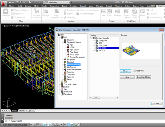
Product Hierarchy Drawing can be dedicated to group parts specifically for FEA
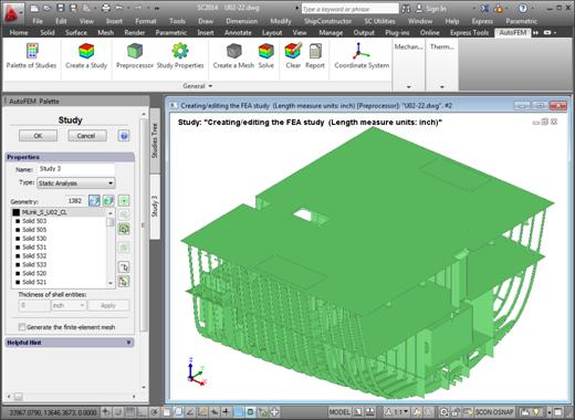
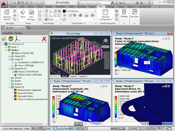
Using the Unit
A Unit drawing may also be used for FEA modelling.
A FEA study addressing a Unit
Use of Assembly
Production drawing (Assemblies, etc.) may be used for finite-element modelling, too.
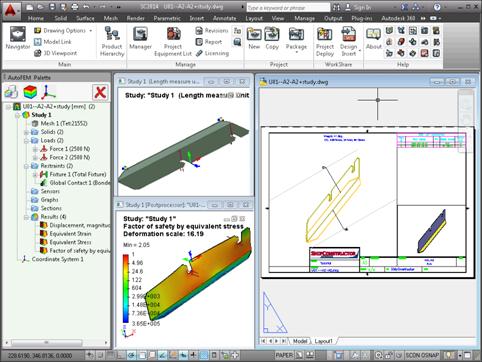
FEA carried out directly on a production assembly
Using the Model Link command
The user may combine several drawings and even Units to create a 3D FEA model, using ShipConstructor's Model Link.
Creating a study encompassing several Units
"Exporting" the 3D model to "external" dwg files
Finally, one can even export a ShipConstructor model to a generic dwg format, and run the FEA outside the ShipCostructor environment.
Finite-element modelling of an "exported" ShipConstructor 3D model
Thus, the ShipConstructor user can choose the most appropriate strategy for his FEA purposes from a variety of options. But, in all cases, without ever leaving the AutoCAD 3D environment.
Settings of integration with ShipConstructor
AutoFEM Analysis is unique in its ability to integrate with the ShipConstructor environment and, most especially, project database. The corresponding functionalities are offered automatically to the user when opening a ShipConstructor drawing.
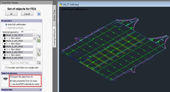
AutoFEM - ShipConstructor integration settings are found in the command dialog "Set of objects for FEA"
The Integration of AutoFEM Analysis with ShipConstructor software includes the following features:
• AutoFEM acquires the ShipConstructor model units, and will use them for FEA;
• AutoFEM acquires the ShipConstructor part names, and uses them to identify the corresponding FE objects in FEA study;
• AutoFEM acquires the mechanical properties of ShipConstructor parts from the project database, for use in FEA (first integration alternative);
• AutoFEM acquires the material name of ShipConstructor parts from the project database and uses the mechanical properties of the material bearing the same name found in the AutoFEM library (second integration alternative).
Let us now more closely consider the two integration alternatives.
1. Direct reading of data from the ShipConstructor materials library using the "take properties from SC base" mode.
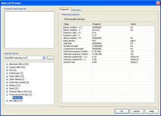
Firstly, the user will specify the mechanical properties of the desired materials in the ShipConstructor project database. For structural strength and buckling analysis, the minimum required set of properties includes the modulus of elasticity (Young's modulus, for example in N/mm2) and Poisson's ratio (dimensionless). For Frequency analysis (calculation of resonance frequencies), material density is required as well.
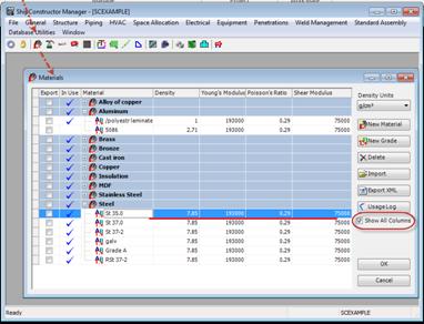
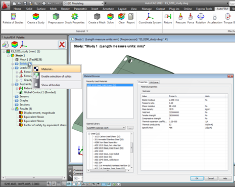
Structural material properties shown in the ShipConstructor database
To facilitate the review and processing of results involving safety factors in static structural FEA, it is also recommended to define, for each material:
• tensile strength,
• compressive strength.
• yield strength (separately for tension and compression, as may be the case),
When "take properties from SC base" is selected, the system will read the material properties from the ShipConstructor project database and will use them for the FEA calculation.
This approach is very powerful for design and scantling sizing work, as material properties are set only once, in the ShipConstuctor project database (and are available to other project databases).
2. Mapping ShipConstructor materials to AutoFEM Analysis materials using the "use AutoFEM materials by name" mode.
The user will ensure that the desired materials in the AutoFEM and ShipConstructor libraries bear the same name. The material properties are then defined only in the AutoFEM library, and these will be used for FEA calculations.
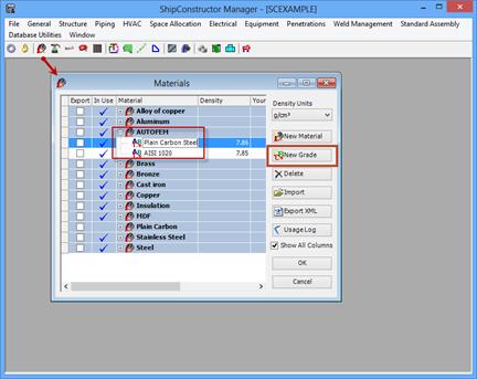
Creating a material whose name is the same in the AutoFEM and ShipConstructor material libraries
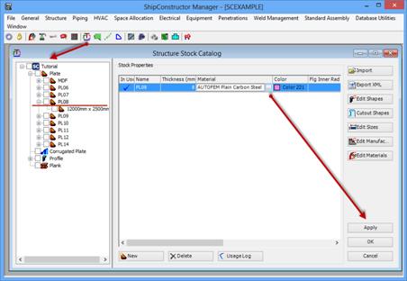
Assigning material to a part in ShipConstructor
This approach is convenient because it allows to use materials with complex properties (e.g., anisotropic) for the analysis of ShipConstructor models, and also to solve the problems of heat conduction and fatigue, in which the nonlinear material properties are not stored in the ShipConstructor material database and in fact can depend on various parameters which identified and quantified during calculation.
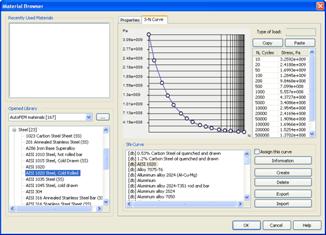
AutoFEM Analysis library of materials allows specifying materials with complex properties
and applying them to ShipConstructor models for FEA.
Stages of finite-element analysis
The typical sequence of an AutoFEM Analysis FEA run includes the following steps:
• Creating a set of objects for finite element study
• Creating the desired study (various types are available)
• Generating the finite element mesh
• Assigning materials (unless already acquired from ShipConstructor
• Defining boundary conditions (constraints, loads)
• Calculation
• Analysis of results
The following paragraphs present the steps listed above, based on a static strength analysis example.
Creating a set of objects for finite element study
The first step involved the creation of the desired objects for finite element study, a set which may include all the model's components, or only some of them. To create the FE objects, the AutoFEM Preprocessor acquires the 3D geometry of the structure from AutoCAD, which is used directly, thereby guaranteeing absolute geometric fidelity.
Only one set of objects for FEA can be defined in a document, and all subsequent studies will be based on this set and use some or all of the objects. Therefore, different studies can involve different groups of objects, all from the same set.
There are two types of object sets:
• set made of 3D solids (AutoCAD 3D solids)
• set made of surface objects (AutoCAD 3D surfaces)
ShipConstructor users will generally work with sets of 3D solid objects, as illustrated below.
In the ShipConstructor drawing, go to the AutoFEM tab and run the "Create a study" command. If the document does not have an existing set of objects for FEA, a dialog appears, to create it.
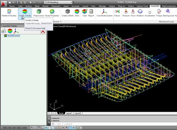
Running the "Create a study" command
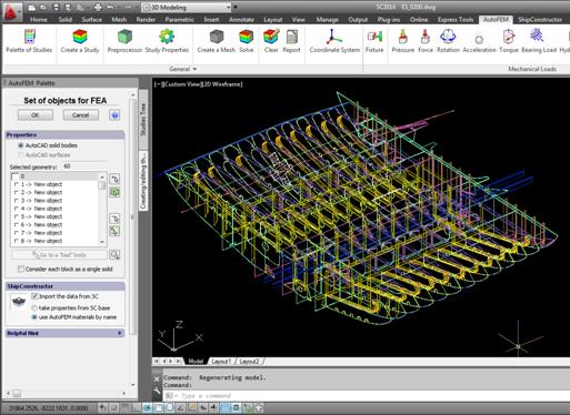
Objects for FEA can be created via the Set of objects for FEA dialog
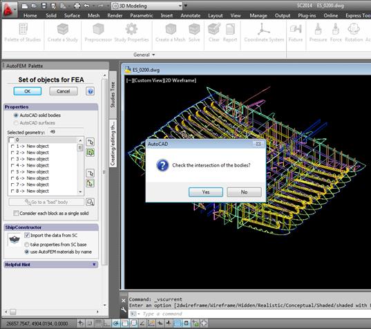
Checking for object / object intersections (clashes)
In order to create the correct and representative FEA mesh, object / object intersections (clashes) must be found and processed. If any are found, the following message appears:
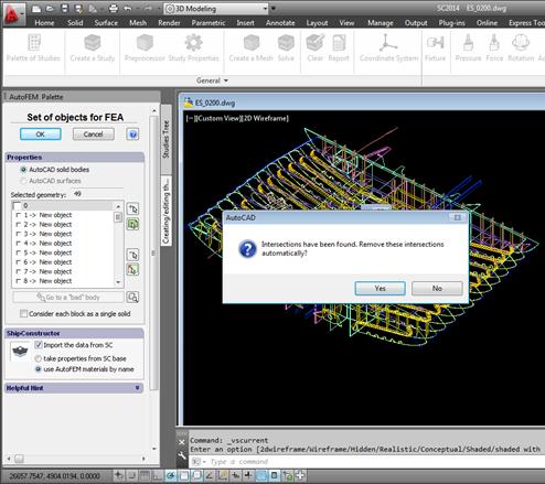
The system offers to automatically fix all object / object intersections
If user refuses the removal of clashes, this may then destroy the mesh generation process. The presence of clashes is admissible in the case when one wants to work with the plate-surface study, based on the faces of 3D solid models. However, volumetric (tetrahedral) meshes foresee that each mesh point belongs to a single object and there are no intersections between 3D solids.
In practice, intersections between objects (clashes) should be avoided when using volumetric FE elements (tetrahedrons).
Once intersections are fixed (eliminated), the study creation process continues.
Creating the desired study
After the successful creation of a set of objects, the command dialog "Creating Study" appears automatically. AutoFEM allows two principal FE formulations:
1. Volumetric formulation: model geometry is approximated with tetrahedral finite elements.
2. Plate (shell) formulation: used in the case of thin-walled structures, the model geometry is approximated with triangular finite elements of plate / shell type. Such formulations are further distinguished as:
• 3D AutoCAD surface models (AutoCAD surfaces);
• 3D AutoCAD solid models, the faces of which are used to build the FE mesh model
The study can include all the objects in the set of objects for FEA, or only some of them, user-selected. The group of objects selected for a study can be modified by adding or removing objects. Studies can be copied, and their type may be modified. For example, one can create and run a Static Analysis study, then change the type to Buckling Analysis and run it again with no further action: objects, boundary conditions, etc. are all persisted. This strategy saves considerable time, eliminates many sources of error, etc.
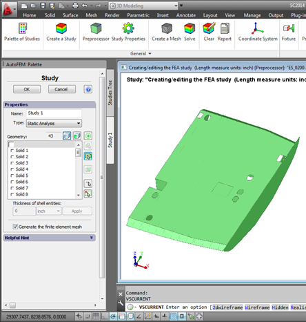
The Study creation dialog
Generating the finite-element mesh
Once the object group of a study is defined, the mesh creation dialog is automatically being available. For models based on 3D solids, a tetrahedral finite element mesh will be generated. For models based on 3D surfaces, AutoFEM will use triangular finite elements.
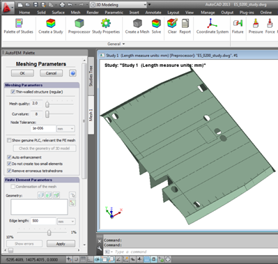
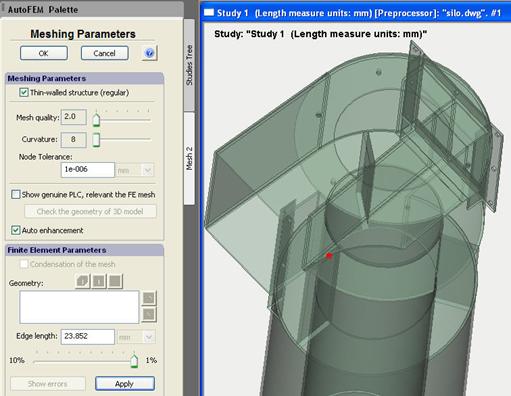
The mesh is created in the Meshing Parameters dialog.
For typical ShipConstructor models, whose parts which are usually relatively thin and spaced apart, it is recommended to build the finite element mesh using the "Thin-walled structure (regular)" option, which will result in a balanced and representative FE mesh. Once the other mesh parameters are selected, the mesh's quality can be evaluated and the creation process completed:
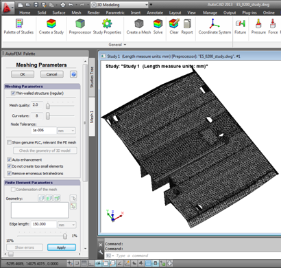
The tetrahedral grid model of a ShipConstructor model
Assigning materials
The AutoFEM Analysis materials library includes the materials most commonly used in various industries. AutoFEM supports anisotropic materials, and allows to set graphs of nonlinear dependence of ultimate strength vs number of loading cycles (SN-curves) for the desired materials.
As noted above, AutoFEM can also acquire material's name directly from the ShipConstructor materials library and add properties only present in the AutoFEM material library (ShipConstructor does not need all strength-related parameters of a given material). In general, if a material is present in the ShipConstructor materials library, its properties should be maintained there.
The AutoFEM materials library
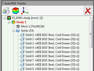
Materials displayed next to the parts' names in each study
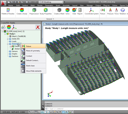
Defining constraints/restraints
FEA generally requires force balancing, hence the model being analyzed must be fixed in space. AutoFEM provided dedicated commands (Fixture, Plane of Symmetry, Elastic base) for this, allowing the specification of a constraint's nature (full or partial). Special filters (selectors) facilitate the selection of the model element(s) to which the constraints are applied: faces, edges, vertices. When required, user coordinate systems are provided to specify the orientation of the degrees of freedom. Constraints are shown graphically on the model.
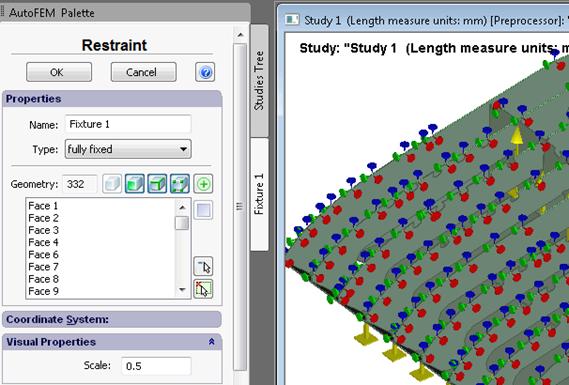
The Restraint dialog
Defining the restraints of a ShipConstructor model
Applying loads
Many different types of loads are available: force, pressure, acceleration, torque hydrostatic load, centrifugal force, and the additional mass. The user determines the magnitude and direction of loads and their application locations. Each load is identified uniquely in the Preprocessor window, and the symbol's size and color are adjustable in the Force dialogue.
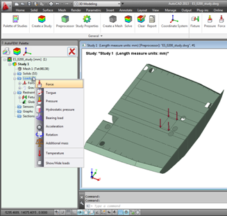
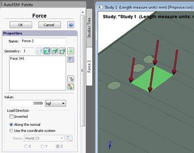
Applying loads to a structural model
The "AutoFEM Palette" lists the defined studies, and each study's pertinent data, mesh characteristics, materials, boundary conditions and calculations results. Additionally, contextual menus are also available for each item in the list. The AutoFEM Palette and the study tree are AutoFEM's principal work management tools.
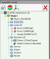
Study Tree, showing the calculation runs
Solving the study
Once the finite element mesh has been created, the materials assigned, restraints and loads imposed, the calculations can be run. Prior to running the calculations, the user selects the equation solving method, a list of results to be made available, and finally specifies additional analysis options which depend on the type of analysis to be run (buckling, nonlinear, thermo-elasticity, etc.).
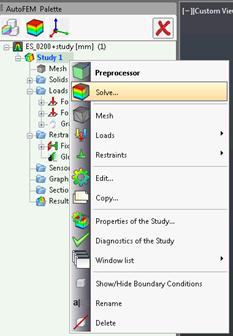
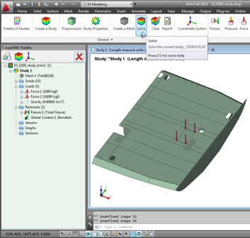
Running calculations from the contextual menu (left) and from the AutoFEM Ribbon (right)
Once the calculation starts, the Study Properties may request additional information specific to that run:
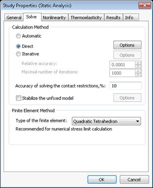
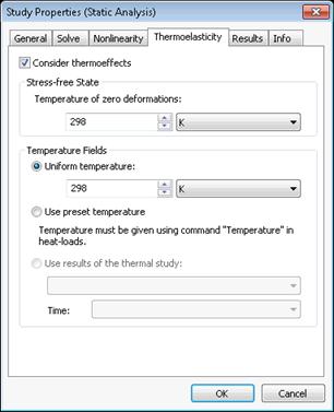
Properties of a Static Analysis study
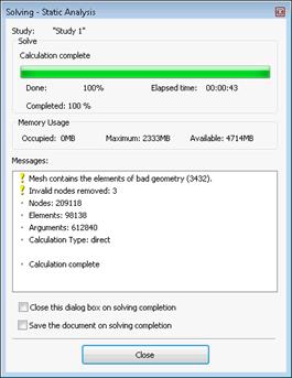
Solving dialog, reporting on calculation status and progress
Studying the results
Once a run completes successfully, the list of results appears in the Study Tree and, from the contextual menu of a given result, the user opens the corresponding Postprocessor window. Results are displayed as color maps directly applied to the structural model, and the user has additional tools available to investigate the results:
· tooltips show the result value as a fly-out
· labels with the result value (double click);
· sensors - special tool to assess results at a preselected point;
· graphics, allowing to reflect changes in the result;
· section, allowing to look into the interior of the model and review results for otherwise invisible points;
· report - creates an independent html-based document, containing the principal results, with color diagrams and 3D VRML models of the results;
· on-screen results animation;
· creating a video of the results animation, in several video-formats;
Review of the color diagrams
In static strength analysis, review of the results begins with the investigation of displacements. The must make sure that the calculated displacements correspond to the expected and have a physical sense. Then, one may proceed to reviewing stresses, etc.
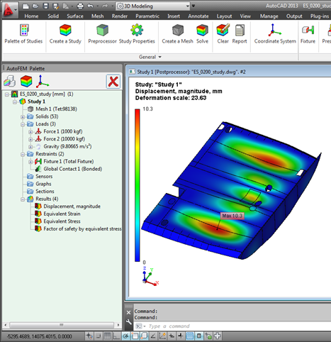
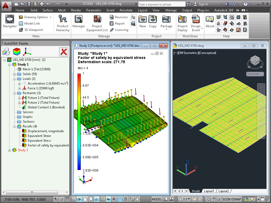
Displaying the calculated deflections
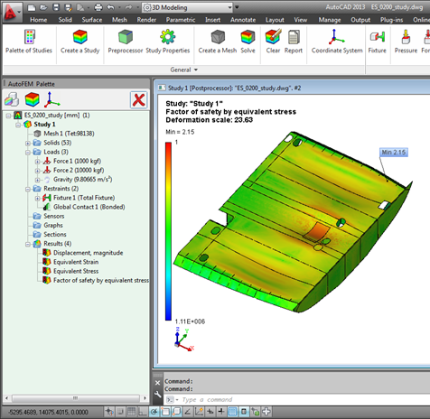
Safety factors expressed as equivalent stress
Animation of the result on-screen
Results can be animated on-screen, one purpose being to review changes due to loading changes.
.
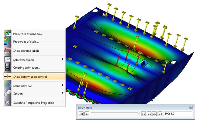
Tools for results animation on-screen
Creating animation videos
The user can create video of the result animations.
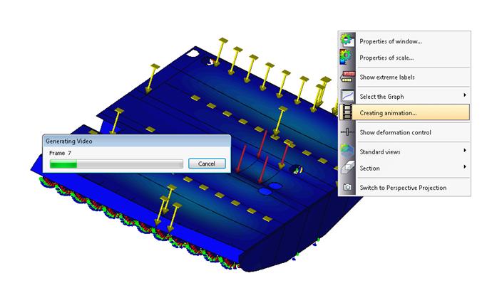
Creating video of animated result
Creating Reports
The "Report" command creates an html document that includes with principal data pertaining to the study at hand. The document can be saved.
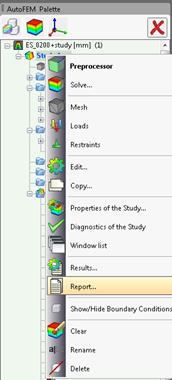
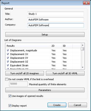
"Report" command in the contextual menu, and its dialog box
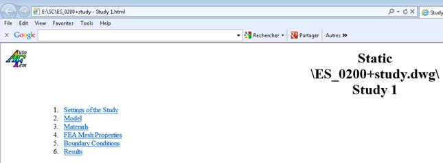
Sections of the report
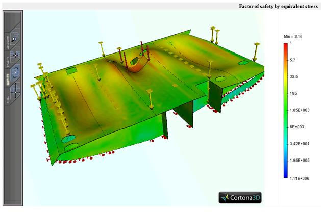
Results overlaid on the 3D model, VRML format, in the html-report
At this point, the user has identified maximum displacements and safety factors, and can ascertain the design's applicability to its intended use. Moreover, presentation materials have been generated, including videos and detailed html-reports.
Conclusion
ShipConstructor this have available a fully integrated, full scope FEA tool to analyze their ShipConstructor models.
For more information on AutoFEM Analysis, please visit autofem.com.
Supplement. Helpful tips and advice
Creating materials in the AutoFEM Analysis material library
As was mentioned earlier in this document, in the ShipConstructor / AutoFEM integrated environment materials can be assigned to structural elements in various ways.
In order to apply material properties found in AutoFEM materials library but in ShipConstructor's, the name of the material at hand must be the same in the two libraries. The steps to ensure this are:
Steps to create a new material:
1. Create a new user’s materials library or open an existing one.
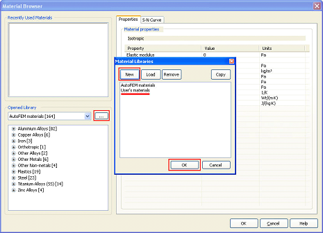
Creating the user’s materials library
2. In the user’s materials library, select an existing group of materials or create a new one.
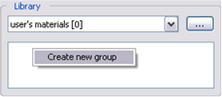
Creating a new group of materials
3. When the cursor is on the group of materials, select "Create a new material" in the context menu.
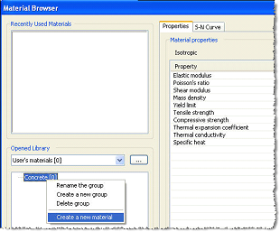
Creating a new material
4. Choose the material type: “Isotropic”, “Orthotropic” or “Transversally isotropic”. Then, enter the name of the material, and click OK. . After OK is pressed, the new material will appear in the current group of materials.
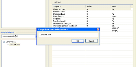
Typing the name of the material
5. Select the newly-created material from the list of materials and fill in its parameters, choosing them from the available selection list
6. Press OK to complete creation of the material and close the dialog.
Validating of the model and fixing intersections
The model's geometry must be checked to make sure it is useable in an FEA exercise. Some of the common problems to look for in AutoCAD models include:
- Intersections (clashes) of 3D solids. Intersecting elements do not model real-life from a FEA standpoint. Any point in a FEA model must belong to a single element or, in our case, physical ShipConstructor part. Sometimes, eliminating intersections may result small changes to the overall 3D geometry, differences which are generally small enough to be negligible. Therefore, the automatic remedying process offered by AutoFEM vastly outweighs the marginally more accurate but also potentially impossible manual correction approach.
Automatic detection and resolving of intersections
Warning!
Intersections are resolved using AutoCAD commands, a process which may require considerable time for very large ShipConstructor models. In extreme cases, AutoCAD may actually crash.
- "Flying" parts. These are objects disconnected from the model, which provoke errors in mechanical studies such as static strength and buckling analysis, but are admissible for frequency and thermal studies.
- Multiple-volume bodies. In terms of FEA meshing, each structure object must subtend a single, closed volume. However, multiple-volume objects can be created in AutoCAD, for example executing a Boolean union on out-of-contact objects, or by creating a solid array, etc. If the AutoFEM tetrahedral modelling strategy is adopted, such instances must be resolved into discrete objects before meshing.
- Out-of-contact solids. Sometimes, it is difficult to determine whether the adjacent faces of solids are indeed touching. This may result in mesh generation or calculation errors. In the interest of clean runs, the users must ensure clear contact between objects.
- Errors in the piece linear complex (PLC) representation of AutoCAD 3D models. These errors may occur in the case of very complex 3D geometry, generally due to 3D modelling operations. Such errors may prevent the creation of a tetrahedral mesh, and the 3D CAD model must be corrected in order to run an FEA.
3Dmodel diagnostics (study)
The Study Diagnostics command is designed to help the user find spurious or FEA-unfit objects in a study object group. The command runs automatically, but it is also available in the Study Tree contextual menu.
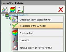
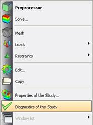
The Diagnostics command in the Set of objects for FEA (left) and Study (right) contextual menus
In all cases, the diagnostics command identifies the spurious objects, which become available in the drop-down "Group of the bodies" list, and whose names are available in the Geometry list.
The following diagnostic modes are available:
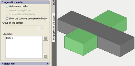
Multiple-volume bodies
· The Multi-volume bodies mode pertains to multiple-volume objects, if any should be present. A Multiple-volume object is one made of two or more solids which do not touch. Which AutoCAD can on contrary treat a single object (body), AutoFEM requires that objects and volumes (bodies) are univocally associated.
Example of a multiple-volume body
The AutoCAD command Explode generally suffices to separate the multiple volumes into discreet objects. In the case where a Boolean operation generated a multiple-volume object, the AutoCAD command SOLIDEDIT/BODY/SEPARATE may be more appropriate if not required.
In some cases, multiple-volume objects may be created during the resolution of intersections by AutoFEM itself. Multiple-volume objects must be resolved into single-volume, discreet object using AutoCAD tools.
Example of a multiple-volume object engendered by the resolution of an intersection,
a condition which must be remedied
Non-contacting groups of bodies
The "out-of-contact bodies" mode addresses objects which are separate from the model. If these objects are not adequately constrained and/or do not bear appropriate boundary conditions, the algebraic system of equations at the heart of FEA may prove to be degenerative, and a solution may not be found. Therefore, in general, such objects should not be included in the Study group of objects in static and buckling analysis, though they are admissible in thermal and frequency analysis studies.
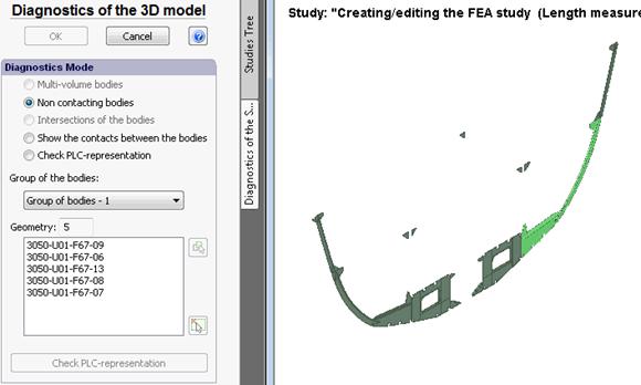
Non contacting parts in the Preprocessor window
Intersecting bodies
· The Intersections of the bodies mode identifies pairs of intersecting objects, which are not allowed in a FE model as a corresponding mesh cannot be created. Although AutoCAD and other CAD systems allow clashing solids, in FEA any point in space must be associated with a single object. Therefore, FEA Incompatible geometry such as this would adversely and unpredictably affect the quality of results, and is not allowed by AutoFEM. The model must be corrected using AutoCAD tools. In addition to AutoFEM's intersection search tools, one may also use AutoCAD's INTERFERE command.
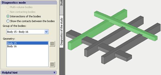
Identifying and documenting pairs of intersecting objects in the diagnostics window
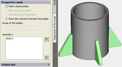
Contact between bodies
· The Show the contacts between the bodies mode identifies all contact faces (two and only two objects share a contact face), which are shown in the pre-processor window. This mode allows the user to check model connections. Sometimes, when modelling in AutoCAD, invisible gaps may occur between objects. These gaps will be treated by AutoFEM as a separation, which will lead to unreliable calculation results. Gaps may also be engendered by the resolving of intersections; making this tool that much more useful and necessary.
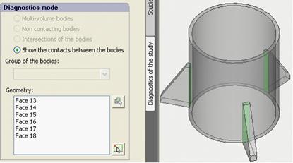
The common faces of contacting parts are shown in green.
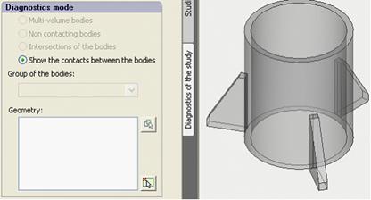
There are no visible contact faces, the modelrequires checking.
Checking the PLC representation
· Check PLC representationchecks the 3D from a PLC standpoint. Inaccuracies are shown in the Pre-processor window; while the "Geometry" window indicates the number of suspicious objects found. These errors are generally remedied by adjusting the mesh construction parameters, otherwise the inaccuracies documented by AutoFEM must be remedied at the model level, in AutoCAD.
·
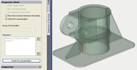
Possible problem areas are highlighted on the model
Note that the FEMAMESH command cannot be run if any multiple-volume bodies are present in the model.
Creating finite-element meshes
It is crucial that the FEA mesh approximates model geometry of the structure very accurately. Sometimes, model modifications are required to achieve a mesh appropriate for structural FEA, in which case the model must be adapted to the purpose.
Moreover, mesh generation parameters may also, on occasion, hamper the generation of a congruent mesh. AutoFEM offer various tools, such as its diagnostics tools, for model reviews and problem area identification.
|
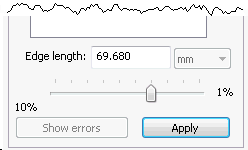
Parameter "Edge length"
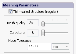
Parameter "Curvature" |
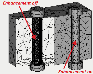
Decreasing the finite element sizeNormally, the system offers too large size of the finite element of mesh. User should define acceptable size of the finite element using a special slider (Edge length) or typing the value in the text box. Increasing the curvature for cylindrical 3D modelsFor 3D models, which have in their composition round or cylindrical geometrical elements, often is useful to increase the accuracy of curve elements representation. Flag Thin-walled structureFlag "Thin-walled structure (regular)" enables a meshing procedure that uses simplified quality control of mesh elements. If the "Mesh quality" parameter is set to "Dis", the mesh will be generated on the basis of the initial PLC model with minimal modifications (usually it looks like a "regular" mesh with square cells). Such meshes contain fewer elements and may be used to compute thin-walled structures, but also in cases where a reduced size mesh is desired. |
Mesh generation errors
If mesh generation should fail, AutoFEM will throw an error message and identify the points and/or geometry area in question. The user can then resolve the problem in the 3D model or exclude the "bad" object(s) from the finite-element study.
Indicating the location of a problem point on the 3D model
Node tolerance for 3D surface models
Nodal coupling tolerance is user controlled, very useful in the case of surface models built on wireframes, which generally exhibit small gaps between surface edges.
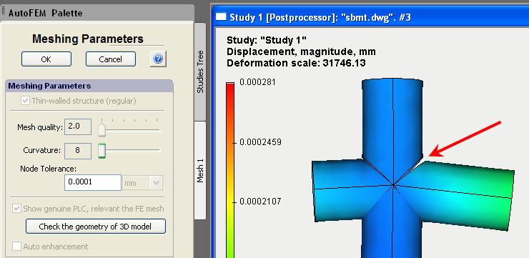
A gap in the mesh model
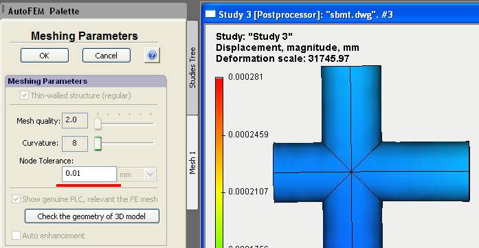
Removing the gaps by increasing the node coupling tolerance
Use of the option "Stabilize the unfixed model"
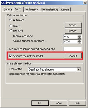
When analysing large ShipConstructor models, it may be that model or element constraints prove inadequate and the model or an element become unbalanced. AutoFEM will then stop calculations and open the following diagnostic message dialogs:
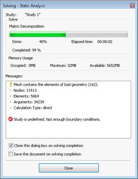
Diagnostic message of unbalanced system
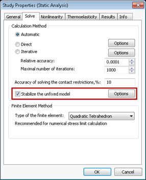
The "Stabilize the unfixed model" tool and its option are found in the Study Properties dialog
Often, the option "Stabilize the unfixed model" helps find inadequately constrained objects or successfully perform the calculation.
Which is the better equation solving method?
The two main methods for the solution of systems of equations are direct and iterative. AutoFEM Analysis will automatically attempt to select the most efficient method for the analysis at hand. If the number of equations exceeds the maximum set in the Processor settings (default 100,000), the iterative method is used for solving. If smaller, the direct method is used. The user can control this choice by defining selection parameters, or by selecting the desired method just prior to launching the analysis.
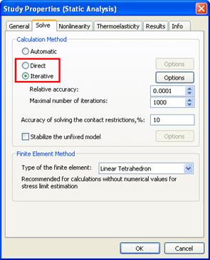
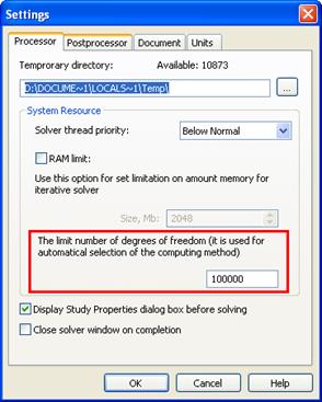
Selecting the system of equation solving method and number of equations threshold
General recommendations and criteria apply to the choice one method or the other.
The first criterion is the power of the computer system. The iterative method requires less RAM than the direct method.
Other criteria are the quality of the finite-element mesh and the "thickness" of the problem.
The direct method is based on the Gauss method and its evolutions, and carries out a full-matrix inversion requiring large amounts of RAM. Calculation time increases as N3, where N =" number "of equations.
Usually the direct method works well and it is preferable when one has:
- A relatively small equation system or a powerful computer system (x64-platform, min 8Gb ram) allowing to invert the FE matrix in RAM (as opposed to using disc swapping). Problems with up to 1.5 -2 million degrees of freedom generally constitute a 'thin" 3D model, and are generally solvable by the direct method
- many of the meshelements are "stretched" (very high aspect ratio)
- the study has contact restrictions
The iterative method's main advantage over the iterative method is its low RAM requirement, which is comparable to the amount of RAM needed for the initial stiffness matrix location. Therefore, even relatively weak computer system (such as an office computer with Windows 32-bit operational system and no more than 3GB RAM) may solve systems of up to 1 million equations or so. On the other hand, performance depends on certain properties of tetrahedral finite elements, such as aspect ratio. And, the more such elements there are, the more solution time will increase, too. Then, the iterative method usually works well and is preferred when one has:
- a good quality mesh where element aspect ratio is less than 8-4 and only few stretched elements.
- "thick" model, meaning that there are several layers of tetrahedral elements per section.
- The study has no contact restrictions.
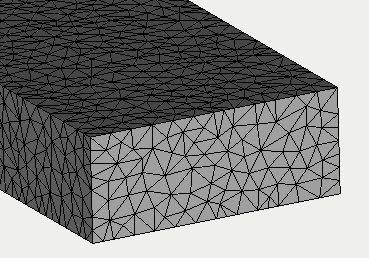
A "thick" finite element model: there are several layers of the finite elements. The Iterative method works better than the direct method for medium and large models.
A "thin" finite element model.The mesh consists of one or two layers of finite elements. The direct method works better than the iterative method, especially if mesh quality is poor (many high aspect ratio mesh elements).
Working with ShipConstructor Pipes
Some ShipConstructor parts, such as pipes, do not have corresponding 3D solid geometry in their ShipConstructor drawing. The user will then export such parts to DWG file, and then simulate them as ordinary after which AutoFEM will treat them as generic AutoCAD objects.
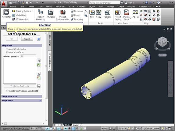
ShipContstructor Pipes do not have 3D solid geometry and cannot be used directly in FEA
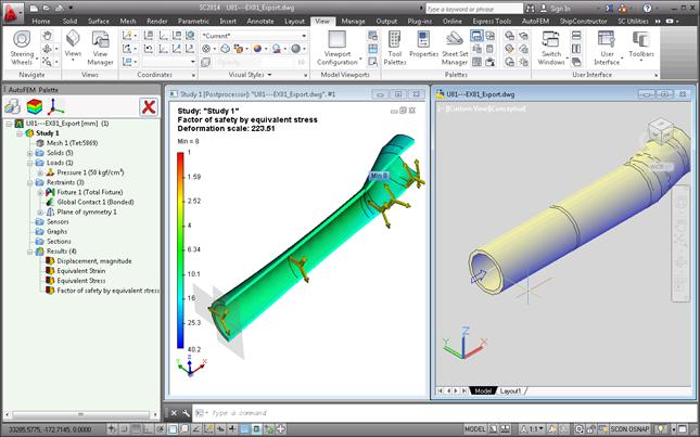
FEA carried out on exported ShipConstructor Pipe parts
AutoFEM Harmonic Forced Oscillations Analysis
Analysis of forced oscillations is performed to predict the behaviour of a structure under external actions which change in accordance with the harmonic law. These actions include force and/or kinematic excitation. In addition to it, the impact of the system damping may be taken into account.

Forced Harmonic Oscillations Analysis
The objective of the forced oscillation analysis is to obtain a dependence of the system’s response on frequency of compelling actions. As a result of calculations we get amplitudes of displacements, vibration acceleration, and vibration overload at the preset compelling frequency. According to these results, one can obtain, for a frequency range, the dependencies of amplitudes and vibration acceleration on frequency of compelling actions, which is important with the evaluation of vibration stability of the system in this preset frequency range.

Phase control of the result
The rotation of a shaft or spindle in the unbalanced state on elastic supports may serve an example of external harmonic force. Kinematic excitation is applied when values of compelling forces are not known, in contrast to amplitudes of oscillations of some structure elements which are known.

Graph of the amplitude-frequency response of the structure
When considering forced oscillations, it is important to take into account the impact of damping forces. The process of energy dissipation of mechanic oscillations, leading to step-by-step attenuation of lump-sum produced oscillations of the system, is termed “damping”. Damping forces may have different origin, namely: friction between dry sliding surfaces, friction between lubricated surfaces, internal friction, air or liquid resistance, etc. It is usually presumed that the damping force is proportional to velocity (viscous damping). Resistance forces changing under the voluntary law are replaced for equivalent damping forces, proceeding from the condition that in one cycle, they dissipate the same amount of energy as real forces.
Dialog of Study's properties
The main results of calculation in the module of forced oscillations are the following values:
- Amplitudes of displacement at finite element mesh nodes Um.
- Vibro accelerations at finite element mesh nodes expressed via amplitudes Um as.
- Vibro overloads, defined as the ratio of vibro acceleration to free fall acceleration.
Below you can find some examples of AutoFEM Forced Oscillations Analysis
|
Verification Examples of AutoFEM Forced Harmonic Oscillations Analysis |
|
|
|
|
|
|
Vibrations of the spring-mass system because of oscillating foundation |
Quick Start (Tutorial) on AutoFEM Forced Oscillations Analysis
Welcome!
This lesson will help you to perform the forced oscillation analysis by the AutoFEM Analysis package.
You will learn to : create a Forced Oscillation Analysis study;
 create the finite element mesh;
 specify a material;
 specify loads and constraints;
 obtain calculation results in the form of colour plots.
Download tutorial video of the AutoFEM Oscillation Analysis Module
Create Forced Oscillation Analysis Study
Step 1: Create Forced Oscillation Analysis Study
Let us consider the mass- spring system (see figure). The plummet is subjected to a harmonic exciting force with amplitude of20 N and phase shift of 30 deg.
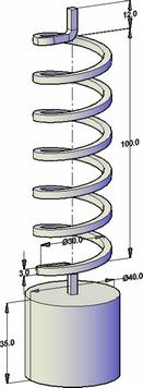
It is necessary to calculate oscillation amplitudes of the mass and phase shifts of the system, using the frequencies, which ranges from 5Hz to 30Hz. The ratios of the Rayleigh damping have following values: ?= 0.02, ?= 3E-004. These values correspond to ~2% of the critical resistance.
To create the Forced Oscillation Analysis problem, we should:
1.Invoke the New problem's properties window using one of the following methods:
|
Command Line: |
FEMASTUDY |
|
Main Menu: |
AutoFEM | Create a Study... |
|
Icon: |
|

2.Select the type of the study ( "Forced Oscillation" ) and add to the list ( "Selected Geometry" ) a solid;
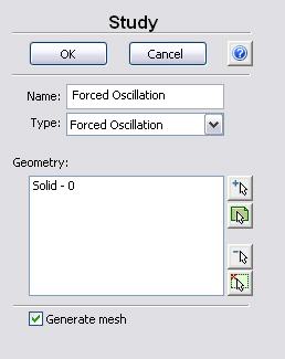
3.Since the option "Generate mesh" is activated, after setting up the problem, the system will automatically proceed to creating finite element mesh;
4". Press  to confirm the New problem creation.
Create Finite Element Mesh
Step 2: Create Finite Element Mesh
After the problem setup, the system automatically proceeds to creating finite element mesh.
To create manually (or modify) the finite element mesh, we need to carry out the following sequence of steps:
1.Invoke the Mesh's properties window by one of the following methods:
|
Command Line: |
FEMAMESH |
|
Main Menu: |
AutoFEM | Create Mesh... |
|
Icon: |
|

2.Let us build the finite-element mesh. The mesh quality is 2, the curvature is 24", the edge length of an element will be no greater than 5.000 mm.
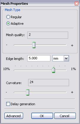
3. Press to complete creating (or modifying) the mesh.
The result of mesh generation is displayed in the 3D window.
Instead of the original model, now you will see the image of the mesh. The original model is not shown at that moment.
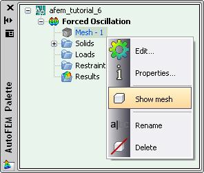
In case it is necessary to hide or display again the finite element mesh, choose the element "Mesh" in the service window "AutoFEM Palette" , then invoke the command "Hide Mesh" or "Show Mesh" from the context menu (by pressing  ).
).
Specify Material
Step 3: Specify the Material
For each problem of the finite element analysis, it is important to correctly specify characteristics of the part's material.
To specify (or modify) the material, we need to carry out the following sequence of steps:
1.Invoke the material's properties window by choosing the folder "Solids" in the service window "AutoFEM Palette" and performing the command "Material..."from the context menu (by pressing  ).
).
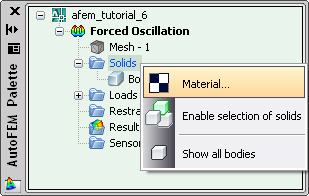
2.Provide a library of materials (into the group "Library");
3.From the list of materials select the material "Plain Carbon Steel" .
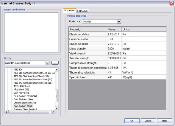
4.Confirm your selection by pressing .
Apply Restraints
Step 4: Apply Restraints
To specify the "Fixed" Restraint , we need to carry out the following sequence of steps:
1. Invoke Restraint's properties window by one of the following methods:
|
Command Line: |
FEMAFIX |
|
Main Menu: |
AutoFEM | Loads\Restrains | Fixture... |
|
Icon: |
 |
2. In the properties window of "Fixture":
a) select the top end of the spring (the flat face) for fixture application;
b) specify the type (“Fully fixed”);
Press to confirm creation.
Apply Loads
Step 5: Apply Loads
To specify the load "Force", we need to carry out the following sequence of steps:
1.Invoke Load's properties window by one of the following methods:
|
Command Line: |
FEMAFORCE |
|
Main Menu: |
AutoFEM | Loads\Restrains | Force... |
|
Icon: |
|

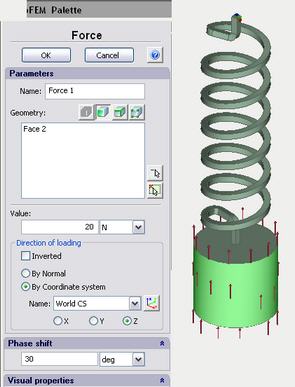
2.In the properties window of "Force":
a)select the cylindrical face of the body for load application;
b)specify the value of force (20 N);
c)specify direction of force (the name of the coordinate system is WorldCS;direction is Z);
d)specify units and the value of the phase shift (in our case the value is equal to 30 deg).
Press to confirm load creation.
Working with the AutoFEM Palette Window
Working with the "AutoFEM Palette" Window
All problems of the document and their components are shown in the service window "AutoFEM Palette" in the form of the structured tree. This window appears automatically after creating the study. If it is necessary, it can be closed or displayed again with the help of the command:
|
Command Line: |
FEMAPAL |
|
Main Menu: |
AutoFEM | Studies Palette |
|
Icon: |
|

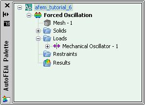
The element "Study" combines all components and objects specified for performing the calculation: finite element mesh ("Mesh"), mechanical loads ("Loads"), constraints ("Restraints").
The folder "Results" is empty until calculation was successfully done.
Solve Study
Step 6: Solve the Study
After constructing the finite element mesh, specifying the loads and restraints, the calculation can be performed.
To solve the problem, the following sequence of steps must be carried out:
1.Invoke the solution's properties window by one of the following methods:
|
Command Line: |
FEMASOLVE |
|
Main Menu: |
AutoFEM | Solve... |
|
Icon: |
|

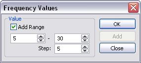
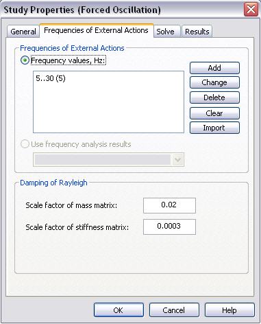
2.On the tab "Parameters", set the option "Frequency values,Hz" and define the range of frequencies (by pressing the button "Add");
3.Set parameters of Rayleigh damping group: the scale factor of mass matrix is equal to 0.02, the scale factor of stiffness matrix is equal to 0.0003.
4.Press , to start calculation.
Customizing Results
After successful solution of the Forced Oscillation Analysis problem, we need to analyze the obtained results.
The list of results available for viewing is shown in the problems tree in the folder "Results".
To extend the list of results shown inthe problems tree, the user has to:
1.From the context menu popping up upon pressing on the name of the selected problem, invoke the window for customizing results (command "Results...");
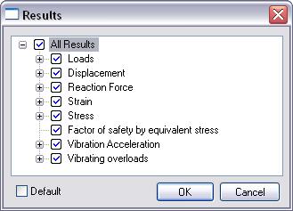
2.Check the results you need;
3.Press .
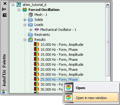
For viewing a result, select it with in the problems window and select the command "Open in new window". The result will be shown in a new window of the Postprocessor.
Analyze Calculation Results
Step 7: Analyze Calculation Results
Let us analyze some important results: “Form, amplitude, mm”, “Form, phase, deg”. We are going to consider these results for the range of the frequencies and graph result-frequency curves.
Let us pay attention to amplitude-frequency dependence.
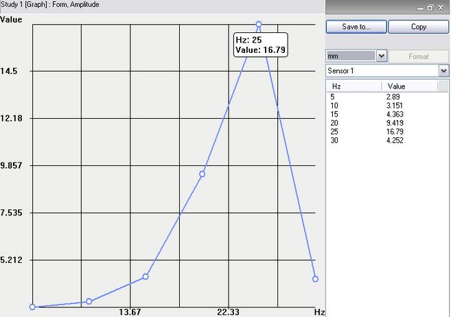
We can see on this diagram that the resonance frequency is about25Hz(to enhance the result a smaller step is needed). To plot points as a smooth curve export the data and paste it to Excel or Mathcad application.
Then let's proceed to phase shift diagram.
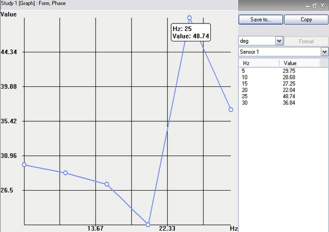
We can see on this diagram that the phase shift (rad) occurs.
Generate Report
Step 8: Generate a Report
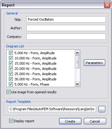
The user can create independent of the AutoFEM Analysis electronic documents which include the main information about the solved problem. The report is created in the html- format.
To create a report, the user needs to:
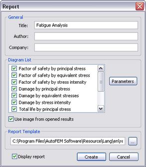
1.Invoke the dialog for customizing a report with the help of the command of the main menu: AutoFEM | Create Report...;
2.Fill in the fields in the group "General";
3.Check the results, which have to be included in the report, in the "Diagram List";
4.Turn on the options "Use image from opened results" and "Display report";
5.Pressing the button  leads to appearance of the dialog for saving the report file.
Congratulations!
You successfully completed the forced oscillation analysis
with the help of the AutoFEM Analysis Lite package.
AutoFEM Fatigue Analysis
The AutoFEM Fatigue Analysis module is used in conjunction with AutoFEM Static Analysis and allows one to evaluate the strength of a structure, which is subjected to cyclic loading. This type of loading is usual in mechanical and structural engineering. The problem is that,when the load is constant, the strength of the structure load may prove to be sufficient. But if this load alternates frequently fatigue of the material occurs and the structure can be damaged or even crushed despite static analysis shows acceptable safety factor. The AutoFEM Fatigue Analysis module allows you to calculate the safety factor depending on the number of loading cycles and on the law of variation of the load's amplitude .

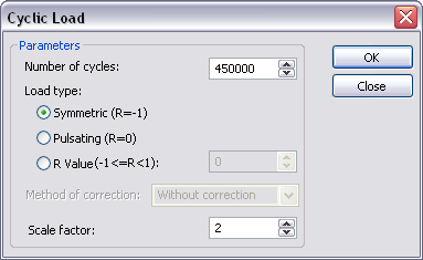
First, it is necessary to solve static study assuming that the loads are constant. Then the user can define cyclic loading parameters in dedicated dialog box of Fatigue Analysis Study. These parameters determine the type of loading (variation law) and number of cycles.
Before running Fatigue Analysis an S-N Curve for the material of the design should be determined. The special S-N Curve Editor is used for this purpose.

A total of 10 results is available in the Fatigue Analysis. They can be divided into four groups.
The group "Damage" includes the following results:
• damage by principal stresses;
• damage by equivalent stresses;
• damage by stress intensity;
The result is displayed in percentage and indicates the damage rate of the structure under the influence of cyclic stresses with the specified number and nature of loading cycles.
The group "Total Life" includes the following results:
• total life by principal stresses;
• total life by equivalent stresses;
• total life by stress intensity.
The result shows the minimum number of cycles Nmin, at which fatigue failure occurs.
The group "Factor of safety" includes results:
• factor of safety by the maximum principal stresses.
• factor of safety by equivalent stresses;
• factor of safety by stress intensity;
The group "Biaxiality". Biaxiality is the ratio of the smaller alternating principal stress (other than zero) to a larger alternating principal stress. The result characterizes inequality of amplitudes of principal stresses at the point and describes the spatial distribution of "unevenness" of the principal stresses in the volume of the body at every point. The value of biaxiality equal to 1 corresponds to the case of state of homogeneous stress? ?at the point.
Note that AutoFEM Fatigue Analysis module is also available in AutoFEM Analysis Lite.
Quick Start on AutoFEM Fatigue Analysis
Welcome!
 Welcome!
This lesson will help you to perform the fatigue analysis by the AutoFEM Analysis Lite package.
You will learn to:
 create a Fatigue Analysis study;
 specify a material; create a S-N curve and associate it with the material;
 define stress cycle parameters ;
 obtain calculation results in the form of colour plots.
Download demo video of the AutoFEM Fatigue Analysis Modul
Analyzing Results of the Static Analysis Study
Step 1: Analyzing results of the Static Analysis study
Let us analyze an model under the static load (i.e. it is necessary to perform calculation of the Static Analysis study) before performing the fatigue analysis.
The results of the Static Analysis study (equivalent stress and principal stress) will be used as stress amplitudes for performing fatigue calculation.
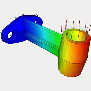
We will take sample model of the bracket and apply "Force".
Let us assume that the load is pulsating. We will try to estimate how many impulsive loading this bracket will stand if applied force is 110 kgf (or 1078.7315 N).
Firstly, we will suppose that the load is static (does not vary with time) and perform calculation of the static analysis study. This type of study has been considered into the Lesson 1 (see AutoFEM Static Analysis).
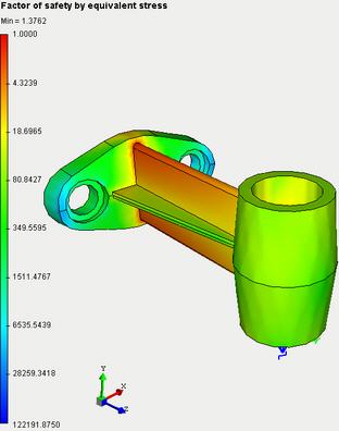
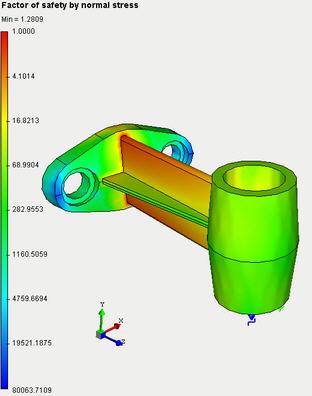
The results of this analysis are given below. Particularly we are interested in:
·factor of safety by equivalent stress (Kmin=" 1.3762);
·factor of safety by normal stress (Kmin= 1.2809);
·factor of safety by shear stress (Kmin= 1.3052).
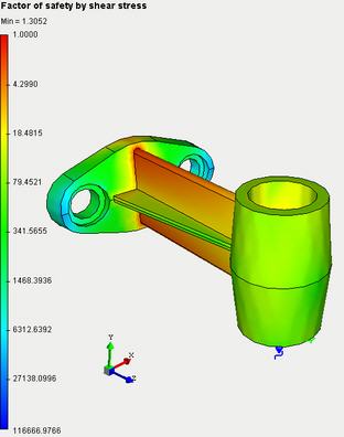
Minimum value of each factor is greater than 1, therefore the part will not fail under static load. Consequently there is sense to analyze this part under cyclically variable loads
Set S-N curve
Step 2: Set S-N curve
Fatigue Analysis requires presence of fatigue curve (S-N curve)for material. AutoFEM Analysis package provides a library of predefined S-N curves for some materials. S-N curve may be selected from the list of predefined curves of the libraryor may be createda new S-N curve in the editor of diagrams.
Tocreate the S-N curvethe user has to do the following steps:
1.Invoke the material properties window by choosing the solid in the service window "AutoFEM Palette" and performing the command "Material..."from the context menu (by pressing  ).
).
2.Provide a library of materials (into the group "Library").
3.Select the material ("Steel AISI 1020") from the list .
4.Press  .
.
5.Define the parameter "Name" and set the value "User defined" for the parameter "Hypothesis";
6.Create nodes for S-N curve with the following coordinates:
|
Number of Cycles |
Maximum Stress, Pa |
|
10 |
3.2592e+009 |
|
20 |
2.4188e+009 |
|
50 |
1.6993e+009 |
|
100 |
1.2845e+009 |
|
200 |
9.8468e+008 |
|
500 |
7".0990e+008 |
|
1000 |
5.5570e+008 |
|
2000 |
4.3727e+008 |
|
5000 |
3.4086e+008 |
|
10000 |
2.9545e+008 |
|
20000 |
2.4169e+008 |
|
50000 |
1.9096e+008 |
|
100000 |
1.6966e+008 |
|
200000 |
1.5254e+008 |
|
500000 |
1.3702e+008 |
|
1000000 |
1.2486e+008 |

7.Check the option "Assign this curve"
8.Press  in the dialog box of material properties.
Create Fatigue Analysis Study
Step 3: Create Fatigue Analysis Study
When you have done whatever is necessary it is able to perform the fatigue analysis successfully.
For creating the Fatigue Analysis study you need to:
1.Invoke the New problem's properties window using one of the following methods:
|
Command Line: |
FEMASTUDY |
|
Main Menu: |
AutoFEM | Create a Study... |
|
Icon: |
|

2.Select option "Fatigue Analysis" for parameter "Type";
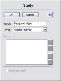
3.Press to confirm creation of the new study.
Set parameters of the fatigue cycle
Step 4: Set Parameters of Fatigue Cycle
For creating the fatigue cycle you need to:
1.Invoke the properties window of the fatigue cycle by choosing the group "Events" in the "AutoFEM Palette" windowand performing the command "Add..."from the context menu (by pressing  ).
).
2.Add already calculated static study;
3.Set parameters of fatigue cycle : number of cycles (N =" 150000), "stress ratio (pulsating, R =" 0), "scale factor (1).
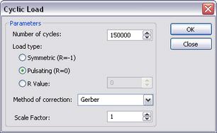
4.Press .
Solve Study
Step 5: Solve the Study
When every parameter of the fatigue cycle is defined it is possible to perform calculation.
Start solving by running appropriate command:
1.Invoke the solution's properties window by one of the following methods:
|
Command Line: |
FEMASOLVE |
|
Main Menu: |
AutoFEM | Solve... |
|
Icon: |
|

2.Press to start calculations.
Customizing Results
After successful completion of fatigue analysis calculation we may analyze the results to make conclusion on fatigue strength with the defined load cycles.
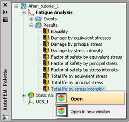
The list of results available for viewing is shown in the study tree in the folder "Results".
Use special dialog box to add or remove results from this list:
1.Press on the study name and run "Results..." command.
2.Select/deselect required items.
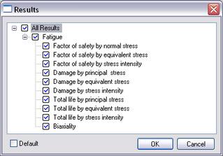
3.Press .
For viewing a result select it by pressing into the "AutoFEM Palette" window and run the command "Open". The result will be shown in a new window of the Postprocessor.
Analyzing Total Life
Step 6: Analyzing Results. Total Life
The total life plot shows that failure due to fatigue is likely to occur after Nmin number of cycles.
The table below shows that the bracket will stand the following number of loading cycles:
|
Total Life |
Number of cycles |
|
- by principal stress |
193825 |
|
- by stress intensity |
247566 |
|
- by equivalent stress |
428637 |
Thus we can see that minimum number of loading cycles that will break the part exceeds required number of cycles (150000) and we can make conclusion about part reliability at the specified cyclic load.
Analyzing the Damage
Step 6: Analyzing Results. Damage
The results for the damage rate indicate what percentage of the life of the model the specified event consumes.
|
Damage |
Damage Rate, % |
|
- by principal stress |
77.39 |
|
- by stress intensity |
60.59 |
|
- by equivalent stress |
34.99 |
Analyzing Safety Factor
Step 6: Analyzing Results. Safety Factor
The safety factor plot indicates that the part will fail due to fatigue if the current loads are multiplied by some value (the minimum safety factor).
In our case the safety factor shows the following values with the current load conditions (R=" 0, "N =" 150000 "cycles).
|
Safety factor |
|
|
- by principal stress |
1.05 |
|
- by stress intensity |
1.07 |
|
- by equivalent stress |
1.14 |
We can see that all three factors are greater than 1, thus we can conclude that the part is reliable with the specified load conditions.
Generate Report
Step 7: Generate a Report
The user can create independent of the AutoFEM Analysis electronic documents which include the main information about the solved problem. The report is created in the html- format.
To create a report, the user needs to:
1.Invoke the dialog for customizing a report with the help of the command of the main menu: AutoFEM | Create Report...;
2.Fill in the fields in the group "General";
3.Check the results, which have to be included in the report, in the "Diagram List";
4.Turn on the options "Use image from opened results" and "Display report";
5.Pressing the button leads to appearance of the dialog for saving the report file.
Congratulations!
You successfully completed the fatigue analysis for the part with the help of the AutoFEM Analysis Lite package.
New features of AutoFEM Analysis 1.4
AutoCAD 2012 now is available. Support of AutoCAD 2012 is included starting from release of the 1.4 version of AutoFEM.

The Installer of AutoFEM Analysis is improved. A special tool is added to control the registration process, in which the AutoCAD version is to be installed in AutoFEM.

New folder "Examples" is added in the AutoFEM Group in the Windows menu “Start|All Programs”. This folder contains files with resolved AutoFEM Studies and allows for a quick understanding of the principles of AutoFEM Analysis by novices.

New verification tests are added to illustrate AutoFEM capabilities of studying systems which have no fixation and are equilibrated by forces or torques.

New features of AutoFEM Analysis 1.3
FEA Processor news
• A new type of the finite-element problem has come to the scene, being harmonic forced oscillations. This type of analysis allows for the calculation of amplitudes of the steady forced oscillations of a mechanical system, on which the harmonic compelling force acts, or at the displacement of the basis in accordance with the harmonic law. The result is amplitudes, accelerations, and overloads, using which may estimate the vibration strength of a structure within the set range of external impacts. This problem type is also available in the AutoFEM Lite version.

A new type of the finite-element problem: forced harmonic oscillations
• The opportunity is added to conduct static analysis for spatially non-fixed bodies, which become equable due to the forces applied. In the previous version of AutoFEM Analysis, to carry out static analysis, the structure was to be necessarily fixed in the space (attached). In the new version, the user may set a mode of “model stabilization” in space, if the original model is not sufficiently fixed.

Calculation of unfixed model equable by forces
• A new type of result is added to the problem of statical analysis: the stress error estimation. This result type permits the estimation of a probability error when calculating the stresses. Most reliable results of the numerical work have a minimum spread of the integral error of the computed stresses.

The Postprocessor window with the result of stress error estimation
• The new type of result is added to the problem of statical analysis: total strength of reaction. It allows one to assess the estimated value of reaction forces, emerging in the structure’s support.

Calculation of reaction forces
• The algorithm of non-linear static analysis (large deformations, geometrical non-linearity) has been improved. Now we have a possibility to solve problems involving general restrictions (Version 1.2 permitted solely "fully fixed" restrictions).
Meshing news
• The algorithm of the work of the generator of finite-element meshs with assemblies has been improved. In particular, the drawback of an earlier algorithm was corrected, including the creation, at assembly structures, of an excessive amount of finite elements that unjustifiably enhanced the dimensionality of the finite-element problem. A new generation mode is a default setting.

Preprocessor news
New types of boundary conditions appeared
• Additional Mass. This command is used only with the load "Acceleration". It allows for a definition, in the system, of additional inert loads coming from a certain massive element of the structure, for instance, as a result of gravitation. We assume thereat that we are not interested in the strained behavior of the massive element per se, but it is necessary to account for its action on other parts of the system. The dimensionality of the problem solved (the number of equations) can be significantly reduced thereat. The Additional Mass can be used in the following studies: static, frequency, and stability analysis, and analysis of forced oscillations.

Using command “Additional mass” for decreasing the problem’s dimensionality
• Elastic base. This type of restraint allows one to define the elastic interaction at the body’s boundary. The elastic base is used to model the touch of the body with the external elastic medium which is deformed together with the body. For instance, the building foundation and the building per se are deformed altogether with the earth on which it stands. Other examples of the body connected with the elastic medium are the dam, railway, etc.

Depiction of the elastic support in the AutoFEM Preprocessor
• Imaging of boundary conditions in the tree of studies has been perfected. Now the value of the applied load is reflected directly in the tree of studies. This essentially eases the perception of conditions of the finite-element problem.

Boundary conditions parameters are reflected in the tree of studies
• Exclusion of the boundary condition from the calculation. A new convenient possibility is added to temporarily exclude any boundary condition (force, restraint, etc.) from the calculation, not removing it in fact The excluded boundary condition is marked by a gray icon in the tree.

Temporary exclusion of the boundary condition from the calculation
• Command “Hide the body” has been updated, which allows one to temporarily hide the body in the Preprocessor window. Now the hidden body is marked by a special icon in the tree of studies. Also, the action of the command applies to all windows of Pre and Postprocessors in AutoFEM.

Retrieval of the command to hide the visibility of the body
• The commands’ interface has been updated. All commands retrieved from the AutoFEM palette now have unfolded bookmarks allowing for space-saving at the display, as well as interactive tip, showing the algorithm of the current command (in the language of the system’s interface). This ensures fast learning of green users.


The new interface of AutoFEM commands
Postprocessor news
• Sensor. A new object has been added for measuring of the result value at the defined point of the finite-element or 3D model. Now every user can define any number of the sensors and use them for analyzing of the results. The sensors are saved in the file .dwg. The sensor can has a multiline commentary which is also saved in the file and which is displayed in the Report of the FEA problem.

Using the sensor for indication of the result value
• Graph. The new type of result is Graph. Using a set of sensors, you can construct the graph of the changing result in the function of dependence across sensors. Besides, the graph for the multiple results can be constructed (for instance, amplitude-frequency characteristic).

The graph of amplitude-frequency characteristic

The set of sensors for measuring the result
Graph constructed using the sensors’ data
• A new convenient tool is added to regulate the model’s orientation in the windows of Preprocessor and Postprocessor. From the context menu in the window of Pre-Postprocessor, the user may select the desirable orientation of the model (similarly to AutoCAD views).

The command for fast control over the model orientation
• The command to construct sections of the model was reworked. Now, you are able to retrieve the command to precisely position the section’s center and orient the plane of the section in space.

Using the command for precise positioning of the section’s plane
• Saving the section’s orientation. The configuration of the section can be saved to ensure the fast access to the set orientation of the section’s planes.
 .
.
Verification Tests news
• The number of verification examples illustrating the exactness of problem solutions was increased twice. Verification problems are now grouped by analysis type that allows for an easy finding of the example using the respective problem class.

Tutorial news
A new lesson aimed at working with module “Forced Harmonic Oscillations” was added.

AutoFEM Thermal Analysis
Using the AutoFEM Thermal Analysis module, any AutoCAD user gets the tool to calculate temperature fields inside mechanic structures. To carry out the thermal problem solving, the 3D model of the item is necessary, which is constructed directly in AutoCAD 3D, or imported into AutoCAD from the other CAD system.
AutoFEM Thermal Analysis permits to carry out the modelling of the thermal fields of two types:
- Stationary thermal fields (the stead-state regime) – the analysed system is steady-state and the temperature distribution does not change with time going on;
- Non-stationary thermal fields – the system is heating or cooling, and the temperature distribution is changing with time passing;
To set the conditions of calculation, different types of boundary conditions are available - temperature, heat flux, convective heat transfer, thermal power. After the calculation is completed, the user can analyse the results using the Post-processor of AutoFEM Analysis, as well as create the independent html-report containing the description of initial data and results of solving the thermal analysis problem.
Below you can find some examples of AutoFEM Thermal Analysis
|
Verification examples of AutoFEM Thermal Analysis |
|
|
|
|
|
|
|
|
|
|
|
|
|
|
|
|
|
|
|
|
|
|
Quick Start on AutoFEM Thermal Analysis
Welcome!
This lesson will help you to perform thermal analysis of the structure with the help of the AutoFEM Analysis Lite.
You will learn to: create a Thermal Analysis problem;
 create a finite element mesh;
 specify materials;
 specify thermal loads;
 perform calculation of stationary temperature fields (steady state regime);
 obtain results of calculation in the form of colour plots.
Download tutorial video of the AutoFEM Thermal Analysis Module
Create Study
Step 1: Create the Thermal Analysis Study
Open the example model to start work.
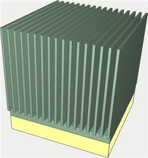
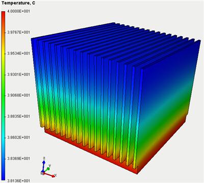
Let us calculate the temperature field for the radiator of the structure "microchip+radiator" shown on the picture. The temperature of the microchip's frame does not exceed 75 oC when the ambient temperature is 25 - 55 oC. For cooling the microchip, the aluminum-alloy radiator secured on the upper part of the microchip's frame is used. The microchip's frame is also made of aluminum for improving heat removal.
To create a Thermal Analysis problem, we need to:
1.Invoke the New problem's properties window using one of the following methods:
|
Command Line: |
FEMASTUDY |
|
Main Menu: |
AutoFEM | Create Study... |
|
Icon: |
|

2.Select the type of the study ( "Thermal Analysis" ) and add to the list ( "Selected Geometry" ) a solid:
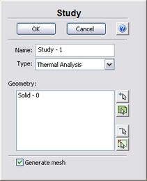
3.Since the option "Generate mesh" is activated, after setting up the problem, the system will automatically proceed to creating finite element mesh;
4.Press  for confirmation of New problem creation.
Create Mesh
Step 2: Create the Finite Element Mesh
After the problem setup, the system automatically proceeds to creating finite element mesh.
To create manually (or modify) the finite element mesh, we need to carry out the following sequence of steps:
1.Invoke the Mesh's properties window by one of the following methods:
|
Command Line: |
FEMAMESH |
|
Main Menu: |
AutoFEM | Create Mesh... |
|
Icon: |
|

2.Let us build the finite-element mesh. The mesh quality will be set as 1.5 .The edge length of an element will be no greater than 4".000 mm .
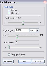
3. Press for completing creation (or modification) of the mesh.
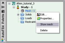
The result of mesh generation is displayed in the 3D window.
Instead of the original model, now you will see the image of the mesh. The original model is not shown at that moment.
In case it is necessary to hide or display again the finite element mesh, choose the element "Mesh" in the service window "AutoFEM Palette" , then invoke the command "Hide Mesh" or "Show Mesh" from the context menu (by pressing  ).
).
Apply Thermal Loads
Step 3: Apply Thermal Loads
For the problem being considered let us specify the following thermal loads. We apply the load "Temperature" equal to 40oC to the bottom face of the radiator, and on the external heat-removing surfaces of the radiator we specify the boundary condition "Convection" with the heat transfer coefficient equal to 15 W/(m2 . oC), and the ambient temperature equal to 25 oC.
To prescribe the load "Temperature", we need to carry out the following sequence of steps:
1.Invoke the Load's properties window by one of the following methods:
|
Command Line: |
FEMATEMP |
|
Main Menu: |
AutoFEM | Loads\Restrains | Temperature... |
|
Icon: |
|

2.In the properties window of the "Temperature":
a) select the face for the load application;
b) specify the magnitude of the load and the units.
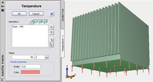
3.Press to confirm creation of the load "Temperature".
To specify the thermal load "Convection" we need to carry out the following sequence of steps:
1.Invoke the Load's properties window by one of the following methods:
|
Command Line: |
FEMACONVECTION |
|
Main Menu: |
AutoFEM | Loads\Restrains | Convection... |
|
Icon: |
|

2.In the properties window of the load "Convection":
a) select the loaded components - faces;
b) specify the heat transfer coefficient, the ambient temperature and the units.
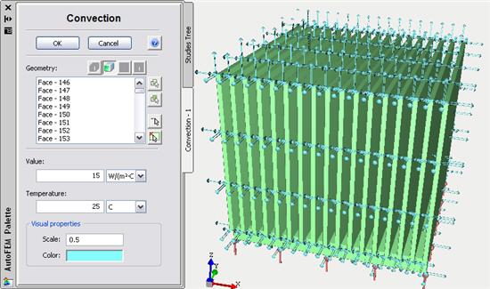
3. Press to confirm creation of the load "Convection".
Specify Material
Step 4: Specify Material
For each problem of the finite element analysis, it is important to correctly specify characteristics of the part's material.
To specify (or modify) the material, we need to carry out the following sequence of steps:
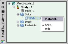
1.Invoke the material's properties window by choosing the solid in the service window "AutoFEM Palette" and performing the command "Material..."from the context menu (by pressing ).
2. Select a library of materials (into the group "Library");
3.From the list of materials, select, for example, "Aluminum Alloy 1060 ";
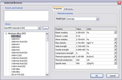
4.Confirm your selection by pressing .
Working with AutoFEM Palette
Working with the "AutoFEM Palette" Window
All problems of the document and their components are shown in the service window "AutoFEM Palette" in the form of the structured tree. This window appears automatically after creating the study. If it is necessary, it can be closed or displayed again with the help of the command:
|
Command Line: |
FEMAPAL |
|
Main Menu: |
AutoFEM | Studies Palette |
|
Icon: |
|

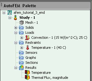
The element "Study" combines all components and objects specified for performing the calculation: finite element mesh ("Mesh"), thermal loads ("Loads").
The folder "Results" is empty until calculation was successfully done.
Solve Study
Step 5: Solve the Thermal Analysis Study
After constructing the finite element mesh, specifying the loads and constraints, the calculation can be performed.
To solve the problem, the following sequence of steps must be carried out:
1.Invoke the solution's properties window by one of the following methods:
|
Command Line: |
FEMASOLVE |
|
Main Menu: |
AutoFEM | Solve... |
|
Icon: |
|

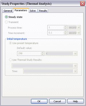
2.On the tab "Parameters", select the option "Steady state";
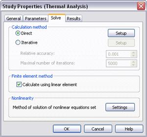
3.On the tab "Solve", in the group "Calculation method" select "Direct", and in the group "Finite element method" turn on the option "Calculate using linear element";
4.Press , to start the calculation.
Customizing Results
Customizing the Results
After successful solution of the Thermal Analysis problem, we need to analyze the obtained results.
The list of results available for viewing is shown in the problems tree in the folder "Results".
To extend the list of results shown in the problems tree, the user has to:
1.From the context menu popping up upon pressing on the name of the selected problem, invoke the window for customizing results (command "Results...");
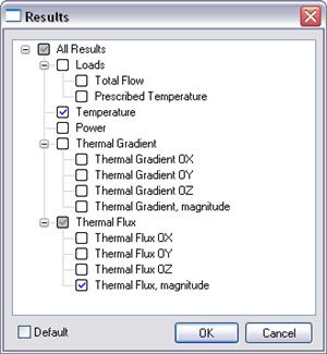
2.Check the results you need;
3".Press .
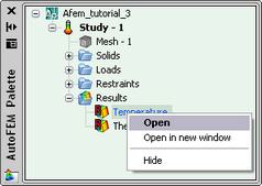
For viewing a result, select it with in the problems window and select the command "Open". You can also use  . The result will be shown in a window of the Postprocessor.
Analyze Calculation Results
Step 6: Analyze Calculation Results
Open the result "Temperature". According to the results of the thermal analysis, the maximum temperature is no greater than 40oC at the temperature of the ambient space equal to 25 oC.
Generate Report
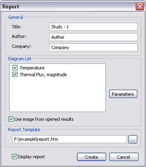
Step 9: Generate a Report
The user can create independent of the AutoFEM electronic documents which include the main information about the solved problem. The report is created in the html- format.
To create a report, the user needs to:
1.Invoke the dialog for customizing a report with the help of the command of the main menu: AutoFEM | Create Report...;
2.Fill in the fields in the group "General";
3.Tick the results, which have to be included in the report, in the "Diagram List";
4.Turn on the options "Use image from opened results" and "Display report";
5.Pressing the button  leads to appearance of the dialog for saving the report file.
Congratulations!
You successfully completed the thermal analysis of the structure with the help of the AutoFEM Analysis.